Determination of the empirical distribution function
Let $X$ be a random variable. $F(x)$ is the distribution function of a given random variable. We will carry out $n$ experiments on a given random variable under the same conditions, independent from each other. In this case, we obtain a sequence of values $x_1,\ x_2\ $, ... ,$\ x_n$, which is called a sample.
Definition 1
Each value $x_i$ ($i=1,2\ $, ... ,$ \ n$) is called a variant.
One estimate of the theoretical distribution function is the empirical distribution function.
Definition 3
An empirical distribution function $F_n(x)$ is a function that determines for each value $x$ the relative frequency of the event $X \
where $n_x$ is the number of options less than $x$, $n$ is the sample size.
The difference between the empirical function and the theoretical one is that the theoretical function determines the probability of the event $X
Properties of the empirical distribution function
Let us now consider several basic properties of the distribution function.
The range of the function $F_n\left(x\right)$ is the segment $$.
$F_n\left(x\right)$ is a non-decreasing function.
$F_n\left(x\right)$ is a left continuous function.
$F_n\left(x\right)$ is a piecewise constant function and increases only at points of values of the random variable $X$
Let $X_1$ be the smallest and $X_n$ the largest option. Then $F_n\left(x\right)=0$ for $(x\le X)_1$ and $F_n\left(x\right)=1$ for $x\ge X_n$.
Let us introduce a theorem that connects the theoretical and empirical functions.
Theorem 1
Let $F_n\left(x\right)$ be the empirical distribution function, and $F\left(x\right)$ be the theoretical distribution function of the general sample. Then the equality holds:
\[(\mathop(lim)_(n\to \infty ) (|F)_n\left(x\right)-F\left(x\right)|=0\ )\]
Examples of problems on finding the empirical distribution function
Example 1
Let the sampling distribution have the following data recorded using a table:
Picture 1.
Find the sample size, create an empirical distribution function and plot it.
Sample size: $n=5+10+15+20=50$.
By property 5, we have that for $x\le 1$ $F_n\left(x\right)=0$, and for $x>4$ $F_n\left(x\right)=1$.
$x value
$x value
$x value
Thus we get:

Figure 2.
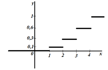
Figure 3.
Example 2
20 cities were randomly selected from the cities of the central part of Russia, for which the following data on public transport fares were obtained: 14, 15, 12, 12, 13, 15, 15, 13, 15, 12, 15, 14, 15, 13 , 13, 12, 12, 15, 14, 14.
Create an empirical distribution function for this sample and plot it.
Let's write down the sample values in ascending order and calculate the frequency of each value. We get the following table:
Figure 4.
Sample size: $n=20$.
By property 5, we have that for $x\le 12$ $F_n\left(x\right)=0$, and for $x>15$ $F_n\left(x\right)=1$.
$x value
$x value
$x value
Thus we get:
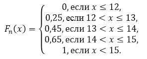
Figure 5.
Let's plot the empirical distribution:
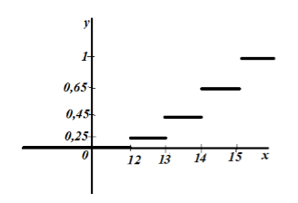
Figure 6.
Originality: $92.12\%$.
Let's study some quantitative trait? general population, and assume that for any sample size the frequency distribution of this characteristic is known. By fixing the sample size to P, denote by p x number of options less than x. Then it is not difficult to see that the relation njn expresses the relative frequency of an event (?
This ratio depends on a fixed number x and, therefore, is some function of this quantity x. Let us denote it by F*(x).
Definition 1.10. Function F*(x) = -, expressing the relative
event frequency (? empirical function
distribution (sampling distribution function or statistical distribution function).
Thus, by definition
Recall that the distribution function of the feature ?, population is defined as the probability of an event (?
![]()
and in contrast to the empirical distribution function is called theoretical distribution function. Since the empirical distribution function is the probability of the same event, then according to Bernoulli’s theorem (see section 5.4), with a large sample size they differ little from each other in the sense that
where e is any arbitrarily small positive number.
Relation (1.2) shows that if the theoretical distribution function is unknown, then the empirical distribution function found from the sample can be used as its sample estimate. From formula (1.2) it simultaneously follows that this estimate is consistent (see Definition 2.4).
Comment 1.6. Attitude nJn can also be interpreted as share those members of the sample that lie to the left of a fixed number x. Let us denote it by co^. Consequently,
Now let's look at an example of constructing an empirical distribution function for a discrete sample.
Example 1.2. The distribution of the sample is known (Table 1.7).
Table 1.7
|
Option x. |
|||||
|
Frequency I. |
Construct its empirical distribution function.
First, let's find the sample size:
Option x x- the smallest. That's why n x = 0 and F*(x)= 0 at X% 3, then P z = 6, i.e. to the left of the point X= 3 there are six sample values. Hence, F*(3) = - = 0.12. To the left x = 5 located
wives n x=5 = 6 + 9= 15 sample option. That's why Fn(5) = - = 0.3. So
How n x=1 = 6 + 9 + 18 = 33, then Fn(7) = - = 0.66. Similarly we find
33 + 12 = 45. Therefore F* (9) = ^ = 0,9.
Option x 5 = 9 is the largest. Therefore, for x > 9, the entire sample lies to the left of this point x. That's why n x>9= 50 and F*(x) = -= 1 for x > 9. 50
Thus, from the calculations carried out above, it follows that the desired empirical function is uniquely defined on the entire real axis, piecewise constant and has the form

The graph of this function represents a step figure and is shown in Fig. 1.6. ?

As for the question of constructing an empirical function for continuous samples, this problem is solved, generally speaking, far from unambiguously. This is due to the fact that the values of the empirical function can be uniquely found only at the end points of partial intervals into which the main interval containing the sample population is divided. But at the interior points of partial intervals it is not defined. At these points it is further determined either by a piecewise constant function (see the previous example) or by some increasing continuous function, for example a linear function, i.e. To construct the empirical distribution function, a linear approximation is used.
Example 1.3. According to Table 1.3, find the empirical distribution function of the enterprise’s employees by length of service.
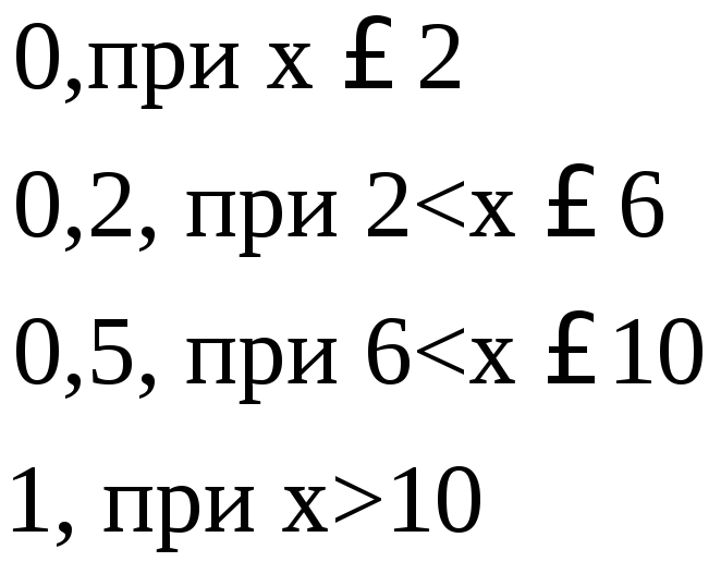
For definiteness, we assume that the partial intervals under consideration are closed on the left and open on the right, i.e. they contain only their left ends. Let x = 2. Then event n 2 = 0 and F*(2)= 0. If x e (2; 6), then at this point the value p x is no longer defined and along with it the value of the empirical function is not defined. For example, if x = 3, then from the conditions of the problem it is impossible to determine the number of workers with less than three years of work experience, i.e. can't find the frequency p x and therefore F*(x).
Further, reasoning in a similar way, we are convinced that the required function F*(x) takes specific values at the left endpoints of partial intervals, for example: "6) = 4/100 = 0.04; "10) = 0.12; "14) = 0.24; "18) = 0.59; F*(22) = 0.78; "26) = 0.90"; "30) = 1, but it is not defined at the interior points of partial intervals. To finally solve the problem, the desired function at the internal points of partial intervals is further defined either by a piecewise constant function (Fig. 1.7) or by some continuous increasing function (Fig. 1.8, where the desired empirical function is extended by a linear function). ?

As is known, the distribution law of a random variable can be specified in various ways. A discrete random variable can be specified using a distribution series or an integral function, and a continuous random variable can be specified using either an integral or a differential function. Let's consider selective analogues of these two functions.
Let there be a sample set of values of some random volume variable  and each option from this set is associated with its frequency. Let further
  is some real number, and
  – number of sample values of the random variable
  , smaller
  .Then the number
  is the frequency of the quantity values observed in the sample X, smaller
  ,
those. frequency of occurrence of the event
,
those. frequency of occurrence of the event  . When it changes x in the general case, the value will also change
  . This means that the relative frequency
  is a function of the argument
  . And since this function is found from sample data obtained as a result of experiments, it is called selective or empirical.
Definition 10.15. Empirical distribution function(sampling distribution function) is the function  , defining for each value x relative frequency of the event
  .
.
 (10.19)
In contrast to the empirical sampling distribution function, the distribution function F(x) of the general population is called theoretical distribution function. The difference between them is that the theoretical function F(x)
determines the probability of an event  , and the empirical one is the relative frequency of the same event. From Bernoulli's theorem it follows
 ,
,
 (10.20)
those. at large  probability
  and relative frequency of the event
  , i.e.
  differ little from one another. From this it follows that it is advisable to use the empirical distribution function of the sample to approximate the theoretical (integral) distribution function of the general population.
Function  And
And  have the same properties. This follows from the definition of the function.
Properties  :
:

Example 10.4. Construct an empirical function based on the given sample distribution:
|
Options | |||
|
Frequencies |


Solution: Let's find the sample size n=
12+18+30=60. Smallest option  , hence,
  at
at  . Meaning
  , namely
  observed 12 times, therefore:
 =
= at
at  .
.
Meaning x<
10, namely  And
And  were observed 12+18=30 times, therefore,
  =
= at
at  . At
. At 
 .
.
The required empirical distribution function:
 =
=
Schedule  shown in Fig. 10.2
R  is. 10.2
Control questions
1. What main problems does mathematical statistics solve? 2. General and sample population? 3. Define sample size. 4. What samples are called representative? 5. Errors of representativeness. 6. Basic methods of sampling. 7. Concepts of frequency, relative frequency. 8. The concept of statistical series. 9. Write down the Sturges formula. 10. Formulate the concepts of sample range, median and mode. 11. Frequency polygon, histogram. 12. The concept of a point estimate of a sample population. 13. Biased and unbiased point estimate. 14. Formulate the concept of a sample average. 15. Formulate the concept of sample variance. 16. Formulate the concept of sample standard deviation. 17. Formulate the concept of sample coefficient of variation. 18. Formulate the concept of sample geometric mean.
Let X 1 , X 2 , ..., X n-- sampling volume P from a population with a distribution function F(x). If you arrange the sample data in non-decreasing order, the resulting series is called variation series: X (1) , X (2) , ..., X (n)
Example 1. If the sample of volume 4 is as follows: 4, -2, 3, 1, then the variation series looks like this: -2, 1, 3, 4.
Definition 1. The empirical distribution function F is called(x) discrete random variable whose distribution table has the following form:
As shown in 2.2.1, the distribution function of a discrete random variable

has the following form:

In other words F n (x) = v/n, Where v--number of those sample values X i , which are smaller X.

As can be seen from the graph, the function F n (x) is stepped and has discontinuities at points X (i) and the magnitude of the jump is 1 /n, if the values coincide with each other X i , No. If k values X (i) coincide, then the magnitude of the jump at this point is equal to k/n.
The limiting behavior is of interest F n (x) at P.
Theorem 1. Let X 1 , X 2 , ..., X n --sample size n from the population by distribution function F(x). Then when n co for any x 1 fair
F n (x) P F(x),
or, in other words, for any > 0,
Proof. Let

discrete random variables such that P( i == 0) = q and P( i = 1) = p, i = 1. 2..... P. It's easy to see that

Then, according to the law of large numbers (see 2.7.2) for the empirical distribution function F n (x) = 1/n n i=1 i at n we get
F n (x) P F(x),
Before formulating another theorem, we give the following definition.
Definition 2. Sequence of random variables 1 , 2 , …, n , … converges to with probability 1 (one) (or almost certainly), if the following equality holds
Now let us formulate (without proof, it can be found in) the following theorem.
Theorem 2 (Glivenko - Cantelli). Under the conditions of the previous theorem, it is true
These results show that at large P the empirical distribution function gives a good approximation to the theoretical distribution function F(x).
Volume samples P from a population with a continuous distribution F(x) in practice they are often subject to grouping. In this case, it is not sample values that are indicated, but the number of sample values that fall within the intervals of some specific partition of the general population (partition of the set of possible values of a random variable that has a distribution function F(x) ). As a rule, intervals are taken of the same length, say h. If we denote by n i number of sample values included in i- interval, then this interval is taken as the base of the height rectangle n i /nh. The resulting figure is called sample histogram. The area of each histogram rectangle is equal to the frequency n i /n the corresponding group. At large P this area will be approximately equal to the probability of falling into the corresponding interval, i.e. will be approximately equal to the integral of the distribution density p( t), calculated over this interval. Thus, the upper part of the histogram contour gives a good approximation for the distribution density.
Example 2. The sensitivity of the 1st channel was tested n = 40 TVs. The test data is shown in the following table, where the first line gives the sensitivity intervals in microvolts, the second - the number of televisions whose sensitivity was found in this interval:

Here the length of the interval h = 50. Let's build a histogram.
ED processing methods are based on the basic concepts of probability theory and mathematical statistics. These include the concepts of general population, sample, empirical distribution function.
Under general population understand all possible parameter values that can be recorded during an unlimited time observation of an object. Such a set consists of an infinite number of elements. As a result of observing an object, a limited-in-volume set of parameter values is formed x 1 , x 2 , …, xn. From a formal point of view, such data represent sample from the general population.
We will assume that the sample contains complete developments before system events (there is no censoring). Observed values x i called options , and their number is sample size n. In order for any conclusions to be drawn from the observation results, the sample must be representative(representative), i.e. correctly represent the proportions of the general population. This requirement is met if the sample size is large enough and each element in the population has the same probability of being included in the sample.
Let the resulting sample have a value x 1 parameter observed n 1 time, value x 2 – n 2 times, meaning xk – nk once, n 1 +n 2 + … +nk=n.
A set of values written in ascending order is called variation series, quantities n i – frequencies, and their relationship to the sample size ni=n i /n – relative frequencies(frequencies). Obviously, the sum of the relative frequencies is equal to unity.
Distribution refers to the correspondence between observed variants and their frequencies or frequencies. Let nx
– the number of observations in which the random values of the parameter X less x. Event Frequency X
distributions: Fn(x) non-decreasing function, its values belong to the segment ;
If x 1 is the smallest value of the parameter, and xk – the greatest, then Fn(x)= 0, When x<x 1 , And FP(xk)= 1 when x>=xk.
Function Fn(x) is determined by ED, which is why it is called empirical distribution function. Unlike the empirical function Fn(x) distribution function F (x) of the population is called the theoretical distribution function, it characterizes not the frequency, but the probability of an event X<x. From Bernoulli's theorem it follows that the frequency Fn(x) tends in probability to probability F(x) with unlimited magnification n. Consequently, with a large volume of observations, the theoretical distribution function F(x) can be replaced by the empirical function Fn(x).
Graph of empirical function Fn(x) is a broken line. In the spaces between adjacent members of the variation series Fn(x) remains constant. When passing through axis points x, equal to the sample members, Fn(x) undergoes a discontinuity, increasing abruptly by the value 1/ n, and if there is a coincidence l observations - on l/n.
Example 2.1. Construct a variation series and graph of the empirical distribution function based on the observation results, table. 2.1.
Table 2.1
The desired empirical function, Fig. 2.1:

Rice. 2.1. Empirical distribution function
With a large sample size (the concept of “large volume” depends on the goals and processing methods, in this case we will consider P big if n>40) for the convenience of processing and storing information resort to grouping EDs into intervals. The number of intervals should be chosen so that the variety of parameter values in the aggregate is reflected to the required extent and at the same time the distribution pattern is not distorted by random frequency fluctuations in individual categories. There are loose guidelines for choosing quantities y And size h such intervals, in particular:
each interval must contain at least 5–7 elements. In extreme ranks, only two elements are allowed;
the number of intervals should not be very large or very small. Minimum the y value must be at least 6 – 7. With a sample size not exceeding several hundred elements, the value y is set in the range from 10 to 20. For a very large sample size ( n>1000) the number of intervals may exceed the specified values. Some researchers recommend using the ratio y=1.441*ln( n)+1;
with relatively small unevenness in the length of the intervals, it is convenient to choose the same and equal to the value
h= (x max – x min)/y,
Where x max – maximum and x min – minimum value of the parameter. If the distribution law is significantly uneven, the length of the intervals can be set to a smaller size in the region of rapid changes in the distribution density;
If there is significant unevenness, it is better to assign approximately the same number of sample elements to each category. Then the length of a particular interval will be determined by the extreme values of the sample elements grouped into this interval, i.e. will be different for different intervals (in this case, when constructing a histogram, normalization by the length of the interval is required - otherwise the height of each element of the histogram will be the same).
Grouping observation results by intervals provides for: determining the range of changes in a parameter X; choosing the number of intervals and their size; counting for everyone i- th interval [ xi–xi+1 ] frequencies ni or relative frequency (frequency n i) options fall into the interval. As a result, a representation of the ED is formed in the form interval or statistical series.
Graphically, a statistical series is displayed in the form of a histogram, polygon and stepped line. Often histogram represented as a figure consisting of rectangles, the bases of which are intervals of length h, and the heights are equal to the corresponding frequency. However, this approach is inaccurate. Height i- th rectangle z i should be chosen equal ni/ (nh). Such a histogram can be interpreted as a graphical representation of the empirical distribution function fn(x), in it the total area of all rectangles will be one. The histogram helps to select the type of theoretical distribution function for approximating the ED.
Polygon called a broken line, the segments of which connect points with coordinates along the abscissa axis equal to the midpoints of the intervals, and along the ordinate axis equal to the corresponding frequencies. The empirical distribution function is displayed as a stepped broken line: a horizontal line segment is drawn over each interval at a height proportional to the accumulated frequency in the current interval. The accumulated frequency is equal to the sum of all frequencies, starting from the first and up to this interval inclusive.
Example 2.2. There are results of recording signal attenuation values xi at a frequency of 1000 Hz of the switched channel of the telephone network. These values, measured in dB, are presented in the form of a variation series in table. 2.3. It is necessary to construct a statistical series.
Table 2.3
| i | |||||||||||
| xi | 25,79 | 25,98 | 25,98 | 26,12 | 26,13 | 26,49 | 26,52 | 26,60 | 26,66 | 26,69 | 26,74 |
| i | |||||||||||
| xi | 26,85 | 26,90 | 26,91 | 26,96 | 27,02 | 27,11 | 27,19 | 27,21 | 27,28 | 27,30 | 27,38 |
| i | |||||||||||
| xi | 27,40 | 27,49 | 27,64 | 27,66 | 27,71 | 27,78 | 27,89 | 27,89 | 28,01 | 28,10 | 28,11 |
| i | |||||||||||
| xi | 28,37 | 28,38 | 28,50 | 28,63 | 28,67 | 28,90 | 28,99 | 28,99 | 29,03 | 29,12 | 29,28 |
Solution. The number of digits of the statistical series should be chosen as minimal as possible to ensure a sufficient number of hits in each of them; let’s take y = 6. Let’s determine the size of the digit
h =(x max – x min)/y =(29.28 – 25.79)/6 = 0.58.
Let's group observations by category, table. 2.4.
Table 2.4
| i | ||||||
| xi | 25,79 | 26,37 | 26,95 | 27,5 3 | 28,12 | 28,70 |
| ni | ||||||
| n i=ni/n | 0,114 | 0,205 | 0,227 | 0,205 | 0,11 4 | 0,136 |
| z i =n i /h | 0,196 | 0,353 | 0,392 | 0,353 | 0,196 | 0,235 |
Based on the statistical series, we will construct a histogram, Fig. 2.2, and the graph of the empirical distribution function, Fig. 2.3.
Graph of the empirical distribution function, Fig. 2.3 differs from the graph presented in Fig. 2.1 equality of the change step of the options and the size of the increment step of the function (when constructed using a variation series, the increment step is a multiple
1/ n, and according to the statistical series - depends on the frequency in a particular category).

The considered ED representations are the initial ones for subsequent processing and calculation of various parameters.