Fourier series expansion of even and odd functions expansion of a function given on an interval into a series in sines or cosines Fourier series for a function with an arbitrary period Complex representation of the Fourier series Fourier series in general orthogonal systems of functions Fourier series in an orthogonal system Minimal property of Fourier coefficients Bessel’s inequality Equality Parseval Closed systems Completeness and closedness of systems


Fourier series expansion of even and odd functions A function f(x), defined on the interval \-1, where I > 0, is called even if the graph of the even function is symmetrical about the ordinate axis. A function f(x), defined on the segment J), where I > 0, is called odd if the graph of the odd function is symmetrical with respect to the origin. Example. a) The function is even on the interval |-jt, jt), since for all x e b) The function is odd, since Fourier series expansion of even and odd functions is expansion of a function given on an interval into a series in sines or cosines Fourier series for a function with an arbitrary period Complex representation of the Fourier series Fourier series for general orthogonal systems of functions Fourier series for an orthogonal system Minimal property of Fourier coefficients Bessel’s inequality Parseval’s equality Closed systems Completeness and closedness of systems c) Function f(x)=x2-x, where does not belong neither to even nor to odd functions, since Let the function f(x), satisfying the conditions of Theorem 1, be even on the interval x|. Then for everyone i.e. /(g) cos nx is even function, and f(x)sinnx is odd. Therefore, the Fourier coefficients of an even function f(x) will be equal. Therefore, the Fourier series of an even function has the form 00 If f(x) - odd function on the interval [-тр, ir|, then the product f(x)cosnx will be an odd function, and the product f(x) sinпх will be an even function. Therefore, we will have Thus, the Fourier series of an odd function has the form Example 1. Expand the function 4 into a Fourier series on the interval -x ^ x ^ n Since this function is even and satisfies the conditions of Theorem 1, then its Fourier series has the form Find the Fourier coefficients. We have Applying integration by parts twice, we obtain that So, the Fourier series of this function looks like this: or, in expanded form, This equality is valid for any x €, since at the points x = ±ir the sum of the series coincides with the values of the function f(x ) = x2, since the graphs of the function f(x) = x and the sum of the resulting series are given in Fig. Comment. This Fourier series allows us to find the sum of one of the convergent numerical series, namely, for x = 0 we obtain that Example 2. Expand the function /(x) = x into a Fourier series on the interval. The function /(x) satisfies the conditions of Theorem 1, therefore it can be expanded into a Fourier series, which, due to the oddness of this function, will have the form Integrating by parts, we find the Fourier coefficients. Therefore, the Fourier series of this function has the form This equality holds for all x B at points x - ±t the sum of the Fourier series does not coincide with the values of the function /(x) = x, since it is equal to. Outside the interval [-*, i-] the sum of the series is a periodic continuation of the function /(x) = x; its graph is shown in Fig. 6. § 6. Expansion of a function given on an interval into a series in sines or cosines Let a bounded piecewise monotonic function / be given on the interval. The values of this function on the interval 0| can be further defined in various ways. For example, you can define a function / on the segment tc] so that /. In this case they say that) “is extended to the segment 0] in an even manner”; its Fourier series will contain only cosines. If the function /(x) is defined on the interval [-l-, mc] so that /(, then the result is an odd function, and then they say that / is “extended to the interval [-*, 0] in an odd way”; in this In this case, the Fourier series will contain only sines. Thus, each bounded piecewise monotonic function /(x) defined on the interval can be expanded into a Fourier series in both sines and cosines. Example 1. Expand the function into a Fourier series: a) by cosines; b) by sines. M This function, with its even and odd continuations into the segment |-x,0) will be bounded and piecewise monotonic. a) Extend /(z) into the segment 0) a) Extend j\x) into the segment (-π,0| in an even manner (Fig. 7), then its Fourier series i will have the form Π = 1 where the Fourier coefficients are equal, respectively for Therefore, b) Extend /(z) into the segment [-x,0] in an odd way (Fig. 8). Then its Fourier series §7. Fourier series for a function with an arbitrary period Let the function fix) be periodic with a period of 21.1 ^ 0. To expand it into a Fourier series on the interval where I > 0, we make a change of variable by setting x = jt. Then the function F(t) = / ^tj will be a periodic function of the argument t with period and it can be expanded on the segment into a Fourier series. Returning to the variable x, i.e., setting, we obtain All theorems valid for Fourier series of periodic functions with period 2π , remain valid for periodic functions with an arbitrary period 21. In particular, a sufficient criterion for the decomposability of a function in a Fourier series also remains valid. Example 1. Expand into a Fourier series a periodic function with a period of 21, given on the interval [-/,/] by the formula (Fig. 9). Because this function is even, then its Fourier series has the form Substituting the found values of the Fourier coefficients into the Fourier series, we obtain We note one thing important property periodic functions. Theorem 5. If a function has period T and is integrable, then for any number a the equality m holds. that is, the integral of a segment whose length is equal to the period T has the same value regardless of the position of this segment on the number axis. In fact, We make a change of variable in the second integral, assuming. This gives and therefore, Geometrically, this property means that in the case of the area shaded in Fig. 10 areas are equal to each other. In particular, for a function f(x) with a period we obtain at Expansion into a Fourier series of even and odd functions, expansion of a function given on an interval into a series in sines or cosines Fourier series for a function with an arbitrary period Complex notation of the Fourier series Fourier series in general orthogonal systems functions Fourier series in an orthogonal system Minimal property of Fourier coefficients Bessel’s inequality Parseval’s equality Closed systems Completeness and closedness of systems Example 2. The function x is periodic with a period Due to the oddness of this function, without calculating integrals, we can state that for any The proven property, in particular, shows , that the Fourier coefficients periodic function f(x) with a period of 21 can be calculated using the formulas where a is an arbitrary real number (note that the functions cos - and sin have a period of 2/). Example 3. Expand into a Fourier series a function given on an interval with a period of 2x (Fig. 11). 4 Let's find the Fourier coefficients of this function. Putting in the formulas we find that for Therefore, the Fourier series will look like this: At the point x = jt (discontinuity point of the first kind) we have §8. Complex representation of the Fourier series This section uses some elements comprehensive analysis(see Chapter XXX, where all actions performed here with complex expressions are strictly justified). Let the function f(x) satisfy sufficient conditions for expansion into a Fourier series. Then on the segment x] it can be represented by a series of the form Using Euler’s formulas Substituting these expressions into series (1) instead of cos πx and sin φx we will have We introduce the following notation Then series (2) will take the form Thus, the Fourier series (1) is represented in complex form (3). Let's find expressions for the coefficients through integrals. We have Similarly, we find The final formulas for с„, с_п and с can be written as follows: . . The coefficients с„ are called the complex Fourier coefficients of the function. For a periodic function with a period), the complex form of the Fourier series will take the form where the coefficients Cn are calculated using the formulas. The convergence of series (3) and (4) is understood as follows: series (3) and (4) are called convergent for given value g, if there are limits Example. Expand the period function into a complex Fourier series. This function satisfies sufficient conditions for expansion into a Fourier series. Let us find the complex Fourier coefficients of this function. We have for odd for even n, or, in short. Substituting the values), we finally obtain Note that this series can also be written as follows: Fourier series for general orthogonal systems of functions 9.1. Orthogonal systems of functions Let us denote by the set of all (real) functions defined and integrable on the interval [a, 6] with a square, i.e., those for which an integral exists. In particular, all functions f(x) continuous on the interval [a , 6], belong to 6], and the values of their Lebesgue integrals coincide with the values of the Riemann integrals. Definition. A system of functions, where, is called orthogonal on the interval [a, b\, if Condition (1) assumes, in particular, that none of the functions is identically zero. The integral is understood in the Lebesgue sense. and we call the quantity the norm of the function. If in an orthogonal system for any n we have, then the system of functions is called orthonormal. If the system (y>„(x)) is orthogonal, then the system Example 1. The trigonometric system is orthogonal on a segment. The system of functions is an orthonormal system of functions on, Example 2. The cosine system and the sine system are orthonormal. Let us introduce the notation that they are orthogonal on the interval (0, f|, but not orthonormal (for I Ф- 2). Since their norms are COS Example 3. Polynomials defined by equality are called Legendre polynomials (polynomials). For n = 0 we have It can be proven , that the functions form an orthonormal system of functions on the interval. Let us show, for example, the orthogonality of the Legendre polynomials. Let m > n. In this case, integrating n times by parts, we find since for the function t/m = (z2 - I)m all derivatives up to order m - I inclusive vanish at the ends of the segment [-1,1). Definition. A system of functions (pn(x)) is called orthogonal on the interval (a, b) by an overhang p(x) if: 1) for all n = 1,2,... there are integrals. Here it is assumed that the weight function p(x) is defined and positive everywhere on the interval (a, b) with the possible exception of a finite number of points where p(x) can vanish. Having performed differentiation in formula (3), we find. It can be shown that the Chebyshev-Hermite polynomials are orthogonal on the interval Example 4. The system of Bessel functions (jL(pix)^ is orthogonal on the interval zeros of the Bessel function Example 5. Let us consider the Chebyshev-Hermite polynomials, which can be defined using equality. Fourier series in an orthogonal system Let there be an orthogonal system of functions in the interval (a, 6) and let the series (cj = const) converge on this interval to the function f(x): Multiplying both sides of the last equality by - fixed) and integrating over x from a to 6, due to the orthogonality of the system, we obtain that this operation has, generally speaking, a purely formal character. However, in some cases, for example, when the series (4) converges uniformly, all functions are continuous and the interval (a, 6) is finite, this operation is legal. But for us now it is the formal interpretation that is important. So, let a function be given. Let us form the numbers c* according to formula (5) and write. The series on the right side is called the Fourier series of the function f(x) with respect to the system (^n(i)). The numbers Cn are called the Fourier coefficients of the function f(x) with respect to this system. The sign ~ in formula (6) only means that the numbers Cn are related to the function f(x) by formula (5) (it is not assumed that the series on the right converges at all, much less converges to the function f(x)). Therefore, the question naturally arises: what are the properties of this series? In what sense does it “represent” the function f(x)? 9.3. Convergence on average Definition. A sequence converges to the element ] on average if the norm is in the space Theorem 6. If a sequence ) converges uniformly, then it converges on average. M Let the sequence ()) converge uniformly on the interval [a, b] to the function /(x). This means that for everyone, for all sufficiently large n, we have Therefore, from which our statement follows. The converse is not true: the sequence () may converge on average to /(x), but not be uniformly convergent. Example. Consider the sequence nx. It is easy to see that But this convergence is not uniform: there exists e, for example, such that, no matter how large n is, on the interval cosines Fourier series for a function with an arbitrary period Complex representation of the Fourier series Fourier series for general orthogonal systems of functions Fourier series for an orthogonal system Minimal property of Fourier coefficients Bessel’s inequality Parseval’s equality Closed systems Completeness and closedness of systems and let We denote by c* the Fourier coefficients of the function /(x ) by an orthonormal system b Consider a linear combination where n ^ 1 is a fixed integer, and find the values of the constants at which the integral takes a minimum value. Let us write it in more detail. Integrating term by term, due to the orthonormality of the system, we obtain. The first two terms on the right side of equality (7) are independent, and the third term is non-negative. Therefore, the integral (*) takes a minimum value at ak = sk. The integral is called the mean square approximation of the function /(x) by a linear combination of Tn(x). Thus, the root mean square approximation of the function /\ takes a minimum value when. when Tn(x) is the 71st partial sum of the Fourier series of the function /(x) over the system (. Setting ak = sk, from (7) we obtain Equality (9) is called the Bessel identity. Since its left side is non-negative, then from it Bessel's inequality follows. Since I am here arbitrarily, Bessel's inequality can be represented in a strengthened form, i.e., for any function / the series of squared Fourier coefficients of this function in an orthonormal system ) converges. Since the system is orthonormal on the interval [-x, m], then inequality (10) translated into the usual notation of the trigonometric Fourier series gives the relation do that is valid for any function /(x) with an integrable square. If f2(x) is integrable, then due to necessary condition convergence of the series on the left side of inequality (11), we obtain that. Parseval's equality For some systems (^„(x)), the inequality sign in formula (10) can be replaced (for all functions f(x) 6 ×) by an equal sign. The resulting equality is called the Parseval-Steklov equality (completeness condition). Bessel's identity (9) allows us to write condition (12) in an equivalent form. Thus, the fulfillment of the completeness condition means that the partial sums Sn(x) of the Fourier series of the function /(x) converge to the function /(x) on average, i.e. according to the norm of space 6]. Definition. An orthonormal system ( is called complete in b2[аy b] if every function can be approximated with any accuracy on average by a linear combination of the form with a sufficiently large number of terms, i.e. if for any function /(x) ∈ b2[a, b\ and for any e > 0 there is natural number nq and numbers a\, a2y..., such that No From the above reasoning follows Theorem 7. If by orthonormalization the system ) is complete in space, the Fourier series of any function / over this system converges to f(x) on average, i.e. by norm It can be shown that the trigonometric system is complete in space. This implies the statement. Theorem 8. If a function /o its trigonometric Fourier series converges to it in average. 9.5. Closed systems. Completeness and closedness of systems Definition. An orthonormal system of functions \ is called closed if in the space Li\a, b) there is no nonzero function orthogonal to all functions. In the space L2\a, b\, the concepts of completeness and closedness of orthonormal systems coincide. Exercises 1. Expand the function 2 into a Fourier series in the interval (-i-, x) 2. Expand the function into a Fourier series in the interval (-tr, tr) 3. Expand the function 4 into a Fourier series in the interval (-tr, tr) into a Fourier series in the interval (-jt, tr) function 5. Expand the function f(x) = x + x into a Fourier series in the interval (-tr, tr). 6. Expand the function n into a Fourier series in the interval (-jt, tr) 7. Expand the function /(x) = sin2 x into a Fourier series in the interval (-tr, x). 8. Expand the function f(x) = y into a Fourier series in the interval (-tr, jt) 9. Expand the function f(x) = | sin x|. 10. Expand the function f(x) = § into a Fourier series in the interval (-π-, π). 11. Expand the function f(x) = sin § into a Fourier series in the interval (-tr, tr). 12. Expand the function f(x) = n -2x, given in the interval (0, x), into a Fourier series, extending it into the interval (-x, 0): a) in an even manner; b) in an odd way. 13. Expand the function /(x) = x2, given in the interval (0, x), into a Fourier series in sines. 14. Expand the function /(x) = 3, given in the interval (-2,2), into a Fourier series. 15. Expand the function f(x) = |x|, given in the interval (-1,1), into a Fourier series. 16. Expand the function f(x) = 2x, specified in the interval (0,1), into a Fourier series in sines.
If the function f(x) has on some interval containing the point A, derivatives of all orders, then the Taylor formula can be applied to it:
Where r n– the so-called remainder term or remainder of the series, it can be estimated using the Lagrange formula:
 , where the number x is between X And A.
If for some value x r n®0 at n®¥, then in the limit the Taylor formula turns into a convergent formula for this value Taylor series:
So the function f(x) can be expanded into a Taylor series at the point in question X, If:
1) it has derivatives of all orders;
2) the constructed series converges at this point.
At A=0 we get a series called near Maclaurin:
Example 1 f(x)= 2x.
Solution. Let us find the values of the function and its derivatives at X=0
f(x) = 2x, f( 0) = 2 0 =1;
f¢(x) = 2x ln2, f¢( 0) = 2 0 ln2= ln2;
f¢¢(x) = 2x ln 2 2, f¢¢( 0) = 2 0 ln 2 2= ln 2 2;
f(n)(x) = 2x ln n 2, f(n)( 0) = 2 0 ln n 2=ln n 2.
Substituting the obtained values of the derivatives into the Taylor series formula, we obtain:
The radius of convergence of this series is equal to infinity, therefore this expansion is valid for -¥<x<+¥.
Example 2 X+4) for function f(x)= e x.
Solution. Finding the derivatives of the function e x and their values at the point X=-4.
f(x)= e x, f(-4) = e -4 ;
f¢(x)= e x, f¢(-4) = e -4 ;
f¢¢(x)= e x, f¢¢(-4) = e -4 ;
f(n)(x)= e x, f(n)( -4) = e -4 .
Therefore, the required Taylor series of the function has the form:
This expansion is also valid for -¥<x<+¥.
Example 3 . Expand a function f(x)=ln x in a series in powers ( X- 1),
(i.e. in the Taylor series in the vicinity of the point X=1).
Solution. Find the derivatives of this function.
![]()
![]()
![]()
![]()
![]()

Substituting these values into the formula, we obtain the desired Taylor series:
Using d'Alembert's test, you can verify that the series converges when
½ X- 1½<1. Действительно,
The series converges if ½ X- 1½<1, т.е. при 0<x<2. При X=2 we obtain an alternating series that satisfies the conditions of the Leibniz criterion. At X=0 function is not defined. Thus, the region of convergence of the Taylor series is the half-open interval (0;2].
Let us present the expansions obtained in this way into the Maclaurin series (i.e. in the vicinity of the point X=0) for some elementary functions:
(2) ![]() ,
,
(3) 
![]() ,
,
( the last decomposition is called binomial series)
Example 4 . Expand the function into a power series
Solution. In expansion (1) we replace X on - X 2, we get:
Example 5
. Expand the function in a Maclaurin series ![]()
Solution. We have ![]()
Using formula (4), we can write:
substituting instead X into the formula -X, we get:

From here we find:
Opening the brackets, rearranging the terms of the series and bringing similar terms, we get
This series converges in the interval
(-1;1), since it is obtained from two series, each of which converges in this interval.
Comment .
Formulas (1)-(5) can also be used to expand the corresponding functions into a Taylor series, i.e. for expanding functions in positive integer powers ( Ha). To do this, it is necessary to perform such identical transformations on a given function in order to obtain one of the functions (1)-(5), in which instead X costs k( Ha) m , where k is a constant number, m is a positive integer. It is often convenient to make a change of variable t=Ha and expand the resulting function with respect to t in the Maclaurin series.
This method illustrates the theorem on the uniqueness of a power series expansion of a function. The essence of this theorem is that in the neighborhood of the same point two different power series cannot be obtained that would converge to the same function, no matter how its expansion is performed.
Example 6 . Expand the function in a Taylor series in a neighborhood of a point X=3.
Solution. This problem can be solved, as before, using the definition of the Taylor series, for which we need to find the derivatives of the function and their values at X=3. However, it will be easier to use the existing expansion (5):

The resulting series converges at ![]() or –3<x- 3<3, 0<x< 6 и является искомым рядом Тейлора для данной функции.
or –3<x- 3<3, 0<x< 6 и является искомым рядом Тейлора для данной функции.
Example 7
. Write the Taylor series in powers ( X-1) functions ![]() .
.
Solution.
The series converges at ![]() , or 2< x£5.
, or 2< x£5.
Which are already pretty boring. And I feel that the moment has come when it is time to extract new canned goods from the strategic reserves of theory. Is it possible to expand the function into a series in some other way? For example, express a straight line segment in terms of sines and cosines? It seems incredible, but such seemingly distant functions can be
"reunification". In addition to the familiar degrees in theory and practice, there are other approaches to expanding a function into a series.
In this lesson we will get acquainted with the trigonometric Fourier series, touch on the issue of its convergence and sum, and, of course, we will analyze numerous examples of the expansion of functions in Fourier series. I sincerely wanted to call the article “Fourier Series for Dummies,” but this would be disingenuous, since solving the problems would require knowledge of other branches of mathematical analysis and some practical experience. Therefore, the preamble will resemble astronaut training =)
Firstly, you should approach the study of page materials in excellent form. Sleepy, rested and sober. Without strong emotions about a broken hamster's leg and obsessive thoughts about the hardships of life for aquarium fish. The Fourier series is not difficult to understand, but practical tasks simply require increased concentration of attention - ideally, you should completely detach yourself from external stimuli. The situation is aggravated by the fact that there is no easy way to check the solution and answer. Thus, if your health is below average, then it is better to do something simpler. Is it true.
Secondly, before flying into space, it is necessary to study the instrument panel of the spacecraft. Let's start with the values of the functions that should be clicked on the machine:
For any natural value:
1) . Indeed, the sinusoid “stitches” the x-axis through each “pi”:
. In the case of negative values of the argument, the result, of course, will be the same: .
2) . But not everyone knew this. The cosine "pi" is the equivalent of a "blinker":
A negative argument does not change the matter: ![]() .
.
Perhaps that's enough.
And thirdly, dear cosmonaut corps, you must be able to... integrate.
In particular, confidently subsume the function under the differential sign, integrate piecemeal and be at peace with Newton-Leibniz formula. Let's begin the important pre-flight exercises. I categorically do not recommend skipping it, so as not to squish in weightlessness later:
Example 1
Calculate definite integrals

where takes natural values.
Solution: integration is carried out over the variable “x” and at this stage the discrete variable “en” is considered a constant. In all integrals put the function under the differential sign:
A short version of the solution that would be good to target looks like this:
Let's get used to it:
The four remaining points are on your own. Try to approach the task conscientiously and write the integrals in a short way. Sample solutions at the end of the lesson.
After performing the exercises QUALITY, we put on spacesuits
and getting ready to start!
Expansion of a function into a Fourier series on the interval
Consider some function that determined at least for a period of time (and possibly for a longer period). If this function is integrable on the interval, then it can be expanded into trigonometric Fourier series:![]() , where are the so-called Fourier coefficients.
, where are the so-called Fourier coefficients.
In this case the number is called period of decomposition, and the number is half-life of decomposition.
It is obvious that in the general case the Fourier series consists of sines and cosines: ![]()
Indeed, let’s write it down in detail:
The zero term of the series is usually written in the form .
Fourier coefficients are calculated using the following formulas: 
I understand perfectly well that those starting to study the topic are still unclear about the new terms: decomposition period, half-cycle, Fourier coefficients etc. Don’t panic, this is not comparable to the excitement before going into outer space. Let’s understand everything in the following example, before executing which it is logical to ask pressing practical questions:
What do you need to do in the following tasks?
Expand the function into a Fourier series. Additionally, it is often necessary to depict a graph of a function, a graph of the sum of a series, a partial sum, and in the case of sophisticated professorial fantasies, do something else.
How to expand a function into a Fourier series?
Essentially, you need to find Fourier coefficients, that is, compose and calculate three definite integral.
Please copy the general form of the Fourier series and the three working formulas into your notebook. I am very glad that some site visitors are realizing their childhood dream of becoming an astronaut right before my eyes =)
Example 2
Expand the function into a Fourier series on the interval. Construct a graph, a graph of the sum of the series and the partial sum.
Solution: The first part of the task is to expand the function into a Fourier series.
The beginning is standard, be sure to write down that:
In this problem, the expansion period is half-period.
Let us expand the function into a Fourier series on the interval: ![]()
Using the appropriate formulas, we find Fourier coefficients. Now we need to compose and calculate three definite integral. For convenience, I will number the points:
1) The first integral is the simplest, however, it also requires eyeballs: 
2) Use the second formula:
This integral is well known and he takes it piece by piece: 
Used when found method of subsuming a function under the differential sign.
In the task under consideration, it is more convenient to immediately use formula for integration by parts in a definite integral  :
:

A couple of technical notes. Firstly, after applying the formula the entire expression must be enclosed in large brackets, since there is a constant before the original integral. Let's not lose her! The parentheses can be expanded at any further step; I did this as a last resort. In the first "piece" ![]() We show extreme care in the substitution; as you can see, the constant is not used, and the limits of integration are substituted into the product. This action is highlighted in square brackets. Well, you are familiar with the integral of the second “piece” of the formula from the training task;-)
We show extreme care in the substitution; as you can see, the constant is not used, and the limits of integration are substituted into the product. This action is highlighted in square brackets. Well, you are familiar with the integral of the second “piece” of the formula from the training task;-)
And most importantly - extreme concentration!
3) We are looking for the third Fourier coefficient:
A relative of the previous integral is obtained, which is also integrates piecemeal:
This instance is a little more complicated, I’ll comment on the further steps step by step: 
(1) The expression is completely enclosed in large brackets. I didn’t want to seem boring, they lose the constant too often.
(2) In this case, I immediately opened these large parentheses. Special attention We devote ourselves to the first “piece”: the constant smokes on the sidelines and does not participate in the substitution of the limits of integration ( and ) into the product . Due to the clutter of the record, it is again advisable to highlight this action with square brackets. With the second "piece" ![]() everything is simpler: here the fraction appeared after opening large parentheses, and the constant - as a result of integrating the familiar integral;-)
everything is simpler: here the fraction appeared after opening large parentheses, and the constant - as a result of integrating the familiar integral;-)
(3) In square brackets we carry out transformations, and in the right integral - substitution of integration limits.
(4) We remove the “flashing light” from the square brackets: , and then open the inner brackets: .
(5) We cancel 1 and –1 in brackets and make final simplifications.
Finally, all three Fourier coefficients are found: ![]()
Let's substitute them into the formula ![]() :
:
At the same time, do not forget to divide in half. At the last step, the constant (“minus two”), which does not depend on “en,” is taken outside the sum.
Thus, we have obtained the expansion of the function into a Fourier series on the interval: ![]()
Let us study the issue of convergence of the Fourier series. I will explain the theory, in particular Dirichlet's theorem, literally "on the fingers", so if you need strict formulations, please refer to the textbook on mathematical analysis (for example, the 2nd volume of Bohan; or the 3rd volume of Fichtenholtz, but it is more difficult).
The second part of the problem requires drawing a graph, a graph of the sum of a series, and a graph of a partial sum.
The graph of the function is the usual straight line on a plane, which is drawn with a black dotted line: 
Let's figure out the sum of the series. As you know, function series converge to functions. In our case, the constructed Fourier series ![]() for any value of "x" will converge to the function, which is shown in red. This function tolerates ruptures of the 1st kind at points, but is also defined at them (red dots in the drawing)
for any value of "x" will converge to the function, which is shown in red. This function tolerates ruptures of the 1st kind at points, but is also defined at them (red dots in the drawing)
Thus: ![]() . It is easy to see that it is noticeably different from the original function, which is why in the entry
. It is easy to see that it is noticeably different from the original function, which is why in the entry ![]() A tilde is used rather than an equals sign.
A tilde is used rather than an equals sign.
Let's study an algorithm that is convenient for constructing the sum of a series.
On the central interval, the Fourier series converges to the function itself (the central red segment coincides with the black dotted line of the linear function).
Now let's talk a little about the nature of the trigonometric expansion under consideration. Fourier series ![]() includes only periodic functions (constant, sines and cosines), so the sum of the series
includes only periodic functions (constant, sines and cosines), so the sum of the series ![]() is also a periodic function.
is also a periodic function.
What does this mean in our specific example? And this means that the sum of the series ![]() –necessarily periodic and the red segment of the interval must be repeated endlessly on the left and right.
–necessarily periodic and the red segment of the interval must be repeated endlessly on the left and right.
I think the meaning of the phrase “period of decomposition” has now finally become clear. To put it simply, every time the situation repeats itself again and again.
In practice, it is usually sufficient to depict three periods of decomposition, as is done in the drawing. Well, and also “stumps” of neighboring periods - so that it is clear that the graph continues.
Of particular interest are discontinuity points of the 1st kind. At such points, the Fourier series converges to isolated values, which are located exactly in the middle of the “jump” of the discontinuity (red dots in the drawing). How to find out the ordinate of these points? First, let’s find the ordinate of the “upper floor”: to do this, we calculate the value of the function at the rightmost point of the central period of the expansion: . To calculate the ordinate of the “lower floor,” the easiest way is to take the leftmost value of the same period: ![]() . The ordinate of the average value is the arithmetic mean of the sum of “top and bottom”: . A pleasant fact is that when constructing a drawing, you will immediately see whether the middle is calculated correctly or incorrectly.
. The ordinate of the average value is the arithmetic mean of the sum of “top and bottom”: . A pleasant fact is that when constructing a drawing, you will immediately see whether the middle is calculated correctly or incorrectly.
Let’s construct a partial sum of the series and at the same time repeat the meaning of the term “convergence.” The motive is also known from the lesson about sum of a number series. Let us describe our wealth in detail:
To compose a partial sum, you need to write zero + two more terms of the series. That is,
In the drawing, the graph of the function is shown in green, and, as you can see, it “wraps” the full sum quite tightly. If we consider a partial sum of five terms of the series, then the graph of this function will approximate the red lines even more accurately; if there are one hundred terms, then the “green serpent” will actually completely merge with the red segments, etc. Thus, the Fourier series converges to its sum.
It is interesting to note that any partial amount is continuous function, however, the total sum of the series is still discontinuous.
In practice, it is not so rare to construct a partial sum graph. How to do it? In our case, it is necessary to consider the function on the segment, calculate its values at the ends of the segment and at intermediate points (the more points you consider, the more accurate the graph will be). Then you should mark these points on the drawing and carefully draw a graph on the period, and then “replicate” it into adjacent intervals. How else? After all, approximation is also a periodic function... ...in some ways its graph reminds me of an even heart rhythm on the display of a medical device.
Carrying out the construction, of course, is not very convenient, since you have to be extremely careful, maintaining an accuracy of no less than half a millimeter. However, I will please readers who are not comfortable with drawing - in a “real” problem it is not always necessary to carry out a drawing; in about 50% of cases it is necessary to expand the function into a Fourier series and that’s it.
After completing the drawing, we complete the task:
Answer: ![]()
In many tasks the function suffers rupture of the 1st kind right during the decomposition period:
Example 3
Expand the function given on the interval into a Fourier series. Draw a graph of the function and the total sum of the series.
![]()
The proposed function is specified in a piecewise manner (and, note, only on the segment) and endures rupture of the 1st kind at point . Is it possible to calculate Fourier coefficients? No problem. Both the left and right sides of the function are integrable on their intervals, therefore the integrals in each of the three formulas should be represented as the sum of two integrals. Let's see, for example, how this is done for a zero coefficient:
The second integral turned out to be equal to zero, which reduced the work, but this is not always the case.
The other two Fourier coefficients are described similarly.
How to show the sum of a series? On the left interval we draw a straight line segment, and on the interval - a straight line segment (we highlight the section of the axis in bold and bold). That is, on the expansion interval, the sum of the series coincides with the function everywhere except for three “bad” points. At the discontinuity point of the function, the Fourier series will converge to an isolated value, which is located exactly in the middle of the “jump” of the discontinuity. It is not difficult to see it orally: left-sided limit: , right-sided limit: ![]() and, obviously, the ordinate of the midpoint is 0.5.
and, obviously, the ordinate of the midpoint is 0.5.
Due to the periodicity of the sum, the picture must be “multiplied” into adjacent periods, in particular, the same thing must be depicted on the intervals and . At the same time, at points the Fourier series will converge to the median values.
In fact, there is nothing new here.
Try to cope with this task yourself. An approximate sample of the final design and a drawing at the end of the lesson.
Expansion of a function into a Fourier series over an arbitrary period
For an arbitrary expansion period, where “el” is any positive number, the formulas for the Fourier series and Fourier coefficients are distinguished by a slightly more complicated argument for sine and cosine:

If , then we get the interval formulas with which we started.
The algorithm and principles for solving the problem are completely preserved, but the technical complexity of the calculations increases:
Example 4
Expand the function into a Fourier series and plot the sum. ![]()
Solution: actually an analogue of Example No. 3 with rupture of the 1st kind at point . In this problem, the expansion period is half-period. The function is defined only on the half-interval, but this does not change the matter - it is important that both pieces of the function are integrable.
Let's expand the function into a Fourier series:
Since the function is discontinuous at the origin, each Fourier coefficient should obviously be written as the sum of two integrals:
1) I will write out the first integral in as much detail as possible:
2) We carefully look at the surface of the Moon:
Second integral take it piece by piece:

What should we pay close attention to after we open the continuation of the solution with an asterisk?
Firstly, we do not lose the first integral  , where we immediately execute subscribing to the differential sign. Secondly, do not forget the ill-fated constant before the big brackets and don't get confused by the signs when using formula
  . Large brackets are still more convenient to open immediately in the next step.
The rest is a matter of technique; difficulties can only be caused by insufficient experience in solving integrals.
Yes, it was not for nothing that the eminent colleagues of the French mathematician Fourier were indignant - how did he dare to arrange functions into trigonometric series?! =) By the way, everyone is probably interested in the practical meaning of the task in question. Fourier himself worked on a mathematical model of thermal conductivity, and subsequently the series named after him began to be used to study many periodic processes, which are visible and invisible in the surrounding world. Now, by the way, I caught myself thinking that it was not by chance that I compared the graph of the second example with the periodic rhythm of the heart. Those interested can familiarize themselves with the practical application Fourier transform in third party sources. ...Although it’s better not to - it will be remembered as First Love =)
3) Taking into account the repeatedly mentioned weak links, let’s look at the third coefficient:
Let's integrate by parts: 

Let us substitute the found Fourier coefficients into the formula ![]() , not forgetting to divide the zero coefficient in half:
, not forgetting to divide the zero coefficient in half:
Let's plot the sum of the series. Let us briefly repeat the procedure: we construct a straight line on an interval, and a straight line on an interval. If the “x” value is zero, we put a point in the middle of the “jump” of the gap and “replicate” the graph for neighboring periods: 
At the “junctions” of periods, the sum will also be equal to the midpoints of the “jump” of the gap.
Ready. Let me remind you that the function itself is by condition defined only on a half-interval and, obviously, coincides with the sum of the series on the intervals
Answer:
Sometimes a piecewise given function is continuous over the expansion period. The simplest example: ![]() . Solution (see Bohan volume 2) the same as in the two previous examples: despite continuity of function at point , each Fourier coefficient is expressed as the sum of two integrals.
. Solution (see Bohan volume 2) the same as in the two previous examples: despite continuity of function at point , each Fourier coefficient is expressed as the sum of two integrals.
On the decomposition interval discontinuity points of the 1st kind and/or there may be more “junction” points of the graph (two, three and generally any final quantity). If a function is integrable on each part, then it is also expandable in a Fourier series. But from practical experience I don’t remember such a cruel thing. However, there are more difficult tasks than those just considered, and at the end of the article there are links to Fourier series of increased complexity for everyone.
In the meantime, let’s relax, lean back in our chairs and contemplate the endless expanses of stars:
Example 5
Expand the function into a Fourier series on the interval and plot the sum of the series.
In this problem the function continuous on the expansion half-interval, which simplifies the solution. Everything is very similar to Example No. 2. There's no escape from the spaceship - you'll have to decide =) An approximate design sample at the end of the lesson, a schedule is attached.
Fourier series expansion of even and odd functions
With even and odd functions, the process of solving the problem is noticeably simplified. And that's why. Let's return to the expansion of a function in a Fourier series with a period of “two pi” ![]() and arbitrary period “two el”
and arbitrary period “two el” ![]() .
.
Let's assume that our function is even. The general term of the series, as you can see, contains even cosines and odd sines. And if we are expanding an EVEN function, then why do we need odd sines?! Let's reset the unnecessary coefficient: .
Thus, an even function can be expanded in a Fourier series only in cosines:
Because the integrals of even functions along an integration segment that is symmetrical with respect to zero can be doubled, then the remaining Fourier coefficients are simplified.
For the gap: 
For an arbitrary interval: 
Textbook examples that can be found in almost any textbook on mathematical analysis include expansions of even functions ![]() . In addition, they have been encountered several times in my personal practice:
. In addition, they have been encountered several times in my personal practice:
Example 6
The function is given. Required:
1) expand the function into a Fourier series with period , where is an arbitrary positive number;
2) write down the expansion on the interval, construct a function and graph the total sum of the series.
Solution: in the first paragraph it is proposed to solve the problem in general form, and this is very convenient! If the need arises, just substitute your value.
1) In this problem, the expansion period is half-period. During further actions, in particular during integration, “el” is considered a constant
The function is even, which means it can be expanded into a Fourier series only in cosines: ![]() .
.
We look for Fourier coefficients using the formulas  . Pay attention to their unconditional advantages. Firstly, the integration is carried out over the positive segment of the expansion, which means we safely get rid of the module
 ![]() , considering only the “X” of the two pieces. And, secondly, integration is noticeably simplified.
, considering only the “X” of the two pieces. And, secondly, integration is noticeably simplified.
Two: 
Let's integrate by parts:


Thus:
, while the constant , which does not depend on “en”, is taken outside the sum.
Answer: 
2) Let’s write down the expansion on the interval; to do this, we substitute the required half-period value into the general formula:
If the function f(x) has derivatives of all orders on a certain interval containing point a, then the Taylor formula can be applied to it:
,
Where r n– the so-called remainder term or remainder of the series, it can be estimated using the Lagrange formula: ![]() , where the number x is between x and a.
, where the number x is between x and a.
Rules for entering functions:
If for some value X r n→0 at n→∞, then in the limit the Taylor formula becomes convergent for this value Taylor series:
,
Thus, the function f(x) can be expanded into a Taylor series at the point x under consideration if:
1) it has derivatives of all orders;
2) the constructed series converges at this point.
When a = 0 we get a series called near Maclaurin:
,
Expansion of the simplest (elementary) functions in the Maclaurin series:
Exponential functions
, R=∞
Trigonometric functions ![]() , R=∞
, R=∞ ![]() , R=∞
, R=∞
, (-π/2< x < π/2), R=π/2
The function actgx does not expand in powers of x, because ctg0=∞
Hyperbolic functions
Logarithmic functions
, -1
Binomial series
![]() .
.
Example No. 1. Expand the function into a power series f(x)= 2x.
Solution. Let us find the values of the function and its derivatives at X=0
f(x) = 2x, f( 0)
= 2 0
=1;
f"(x) = 2x ln2, f"( 0)
= 2 0
ln2= ln2;
f""(x) = 2x ln 2 2, f""( 0)
= 2 0
ln 2 2= ln 2 2;
…
f(n)(x) = 2x ln n 2, f(n)( 0)
= 2 0
ln n 2=ln n 2.
Substituting the obtained values of the derivatives into the Taylor series formula, we obtain:
The radius of convergence of this series is equal to infinity, therefore this expansion is valid for -∞<x<+∞.
Example No. 2. Write the Taylor series in powers ( X+4) for function f(x)= e x.
Solution. Finding the derivatives of the function e x and their values at the point X=-4.
f(x)= e x, f(-4)
= e -4
;
f"(x)= e x, f"(-4)
= e -4
;
f""(x)= e x, f""(-4)
= e -4
;
…
f(n)(x)= e x, f(n)( -4)
= e -4
.
Therefore, the required Taylor series of the function has the form:
This expansion is also valid for -∞<x<+∞.
Example No. 3. Expand a function f(x)=ln x in a series in powers ( X- 1),
(i.e. in the Taylor series in the vicinity of the point X=1).
Solution. Find the derivatives of this function.
f(x)=lnx , , , , ![]()
![]()
f(1)=ln1=0, f"(1)=1, f""(1)=-1, f"""(1)=1*2,..., f (n) =(- 1) n-1 (n-1)!
Substituting these values into the formula, we obtain the desired Taylor series:
Using d'Alembert's test, you can verify that the series converges at ½x-1½<1 . Действительно,
The series converges if ½ X- 1½<1, т.е. при 0<x<2. При X=2 we obtain an alternating series that satisfies the conditions of the Leibniz criterion. When x=0 the function is not defined. Thus, the region of convergence of the Taylor series is the half-open interval (0;2].
Example No. 4. Expand the function into a power series. Example No. 5. Expand the function in a Maclaurin series Comment
.
This method is based on the theorem on the uniqueness of the expansion of a function in a power series. The essence of this theorem is that in the neighborhood of the same point two different power series cannot be obtained that would converge to the same function, no matter how its expansion is performed. Example No. 5a. Expand the function in a Maclaurin series and indicate the region of convergence. The fraction 3/(1-3x) can be considered as the sum of an infinitely decreasing geometric progression with a denominator of 3x, if |3x|< 1. Аналогично, дробь 2/(1+2x) как сумму бесконечно убывающей геометрической прогрессии знаменателем -2x, если |-2x| < 1. В результате получим разложение в степенной ряд
Example No. 6. Expand the function into a Taylor series in the vicinity of the point x = 3. Example No. 7. Write the Taylor series in powers (x -1) of the function ln(x+2) . Example No. 8. Expand the function f(x)=sin(πx/4) into a Taylor series in the vicinity of the point x =2. Example No. 1. Calculate ln(3) to the nearest 0.01. Example No. 2. Calculate to the nearest 0.0001. Example No. 3. Calculate the integral ∫ 0 1 4 sin (x) x to within 10 -5 . Example No. 4. Calculate the integral ∫ 0 1 4 e x 2 with an accuracy of 0.001.
Solution. In expansion (1) we replace x with -x 2, we get:
, -∞![]() .
.
Solution. We have
Using formula (4), we can write:
substituting –x instead of x in the formula, we get:
From here we find: ln(1+x)-ln(1-x) = -
Opening the brackets, rearranging the terms of the series and bringing similar terms, we get
. This series converges in the interval (-1;1), since it is obtained from two series, each of which converges in this interval.
Formulas (1)-(5) can also be used to expand the corresponding functions into a Taylor series, i.e. for expanding functions in positive integer powers ( Ha). To do this, it is necessary to perform such identical transformations on a given function in order to obtain one of the functions (1)-(5), in which instead X costs k( Ha) m , where k is a constant number, m is a positive integer. It is often convenient to make a change of variable t=Ha and expand the resulting function with respect to t in the Maclaurin series.
Solution. First we find 1-x-6x 2 =(1-3x)(1+2x) , . ![]() to elementary:
to elementary:
with convergence region |x|< 1/3.
Solution. This problem can be solved, as before, using the definition of the Taylor series, for which we need to find the derivatives of the function and their values at X=3. However, it will be easier to use the existing expansion (5):
=
The resulting series converges at or –3
Solution.
The series converges at , or -2< x < 5.
Solution. Let's make the replacement t=x-2:
Using expansion (3), in which we substitute π / 4 t in place of x, we obtain:
The resulting series converges to the given function at -∞< π / 4 t<+∞, т.е. при (-∞
, (-∞Approximate calculations using power series
Power series are widely used in approximate calculations. With their help, you can calculate the values of roots, trigonometric functions, logarithms of numbers, and definite integrals with a given accuracy. Series are also used when integrating differential equations.
Consider the expansion of a function in a power series:
In order to calculate the approximate value of a function at a given point X, belonging to the region of convergence of the indicated series, the first ones are left in its expansion n members ( n– a finite number), and the remaining terms are discarded:
To estimate the error of the obtained approximate value, it is necessary to estimate the discarded remainder rn (x) . To do this, use the following techniques:
Solution. Let's use the expansion where x=1/2 (see example 5 in the previous topic):
Let's check whether we can discard the remainder after the first three terms of the expansion; to do this, we will evaluate it using the sum of an infinitely decreasing geometric progression:
So we can discard this remainder and get
Solution. Let's use the binomial series. Since 5 3 is the cube of an integer closest to 130, it is advisable to represent the number 130 as 130 = 5 3 +5. 
since already the fourth term of the resulting alternating series satisfying the Leibniz criterion is less than the required accuracy:
, so it and the terms following it can be discarded.
Many practically necessary definite or improper integrals cannot be calculated using the Newton-Leibniz formula, because its application is associated with finding the antiderivative, which often does not have an expression in elementary functions. It also happens that finding an antiderivative is possible, but it is unnecessarily labor-intensive. However, if the integrand function is expanded into a power series, and the limits of integration belong to the interval of convergence of this series, then an approximate calculation of the integral with a predetermined accuracy is possible.
Solution. The corresponding indefinite integral cannot be expressed in elementary functions, i.e. represents a “non-permanent integral”. The Newton-Leibniz formula cannot be applied here. Let's calculate the integral approximately.
Dividing term by term the series for sin x on x, we get: 
Integrating this series term by term (this is possible, since the limits of integration belong to the interval of convergence of this series), we obtain:
Since the resulting series satisfies Leibniz’s conditions and it is enough to take the sum of the first two terms to obtain the desired value with a given accuracy.
Thus, we find  .
.
Solution.

![]() . Let's check whether we can discard the remainder after the second term of the resulting series.
. Let's check whether we can discard the remainder after the second term of the resulting series.
0.0001<0.001. Следовательно, 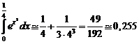 .
.