Function approximation several independent variables (multiple regression) is a very interesting task with great practical importance! If you learn how to solve it, you can become almost a wizard, able to make very reliable predictions...
Results of various processes based on data from previous periods of time. In this article we will look at forecasting in Excel using a very powerful and convenient tool— built-in statistical functions LINEST and LGRFPRIBL.
Don't be intimidated by the "clever" terms! Everything is actually not as scary as it seems at first! Take your time and read this article carefully to the end. The ability to put these functions into practice will significantly increase your “weight” as a specialist in the eyes of colleagues, managers and in your own eyes!
One of the most popular articles on this blog talks about it in detail (I recommend reading it). But in real life processes the result, as a rule, depends on many independent factors (variables) from each other. How to identify and take into account all these factors, connect them together and, based on accumulated statistical data, predict the final result for a certain new set of initial parameters? How to assess the reliability of the forecast and the degree of influence of each variable on the result? Answers to these and other questions are further in the text of the article.
What can you learn to predict? A lot of things! In principle, you can learn to predict any wide variety of process results in Everyday life and work. Whenever the question arises: “What will happen if...?” Call Excel for help, calculate the forecast and check its accuracy!
You can learn to predict the dependence of profit on the price and sales volume of any product.
You can learn to predict the dependence of the price of cars on the secondary market on the brand, power, configuration, year of manufacture, number of previous owners, mileage.
You can learn to establish the dependence of sales volumes of goods on the costs of different kinds advertising.
You can learn how to forecast in Excel the cost of sets of any services depending on their composition and quality.
In production, using indirect simple parameters, you can learn to predict labor intensity and volume of products, consumption of materials and energy resources, etc.
Before starting to solve a practical problem, I want to draw your attention to one very important point. Learning to perform forecasting in Excel using the above-mentioned LINEST and LGRFPRIBL functions is not technically very difficult. It is much more difficult to learn to analyze the process leading to the result and find simple factors influencing it. In this case, it is desirable (but not necessary) to understand HOW the result (function) depends on each of the factors (variables). Is this a linear relationship or maybe a power law or some other kind? Understanding physical meaning process will help you choose the right variables. The selection of the approximating function should be made with a full understanding of the logic and meaning of the process leading to the result.
Preparing for forecasting in Excel.
1. We clearly formulate the name and unit of measurement of the process result that interests us. This is the required function - y, the analytical expression of which we will determine using MS Excel.
In the example below, y— this is the order production time in working days.
2. We analyze the process and identify factors - function arguments - x 1 , x 2 , ... x n— the ones that most strongly influence the result, in our opinion, are the function values y. We carefully assign units of measurement for variables.
In the example this is:
x 1— the total length of all rolled profiles in meters from which the order is made
x 2— total mass of all rolled profiles in kilograms
x 3- total area of all sheets in square meters
x 4- total mass of all sheets in kilograms
3. We collect statistics - actual data - in the form of a table.
In the example, this is actual data on rolled metal and the actual timing of previously completed orders.
Very important when choosing variables x 1 , x 2 , ... x n take into account their availability. That is, you should have the values of these factors in the form of reliable statistical data. It is highly desirable that obtaining statistical data values be a simple, understandable and non-labor-intensive process.
Let's move on to the example.
A small section of the plant produces structural metal structures. The input raw materials are sheet and profile metal products. The thickness of the site in the time period under consideration is unchanged. There are statistical data available on the production time of 13 orders ( k=13) and the amount of rolled metal used. Let's try to find the dependence of the order production time on the total length and weight of rolled profiles and the total area and weight of rolled sheets.
In the example considered, the order production time directly depends on production capacity (people, equipment) and the labor intensity of technological operations. But detailed technological calculations are very labor-intensive and, accordingly, time-consuming and expensive. Therefore, four parameters were selected as arguments to the function, which can be easily and quickly calculated if you have a rolled metal specification, and which indirectly affect the result - the production time. As a result of the analysis, a strong connection was established between changes in the initial data and the results of the metal structures manufacturing process.
It is noteworthy that the found dependence connects the parameters with different units measurements. This is fine. The found coefficients are not dimensionless. For example, the dimension of the coefficient b– working days, and the coefficient m 1 – working days/m.
1. Launch MS Excel and fill cells B4...F16 of the Excel table with initial statistical data. We write the values of variables in the columns x i and actual function values y, placing data related to one order on one line.

2. Since the LINEST and LGRFPRIBL functions are functions that output results as an array, then their input has some peculiarities. We select an area of 5x5 cells - cells I9...M13. The number of allocated rows is always 5, and the number of columns must be equal to the number of variables x i plus 1. In our case it is: 4+1=5.
3. Press the F2 key on the keyboard and enter the formula
in cells I9...M13: =LINEST(F4:F16,B4:E16,TRUE,TRUE)
4. After typing the formula, you must press the key combination Ctrl+Shift+Enter to enter it. (The “+” sign does not need to be pressed; in writing, it means that the keys are pressed sequentially while holding down all the previous ones.)
5. We read the results of the LINEST function in cells I9...M13.
I placed a map explaining the values of which parameters are displayed in which cells in cells I4...M8 for ease of reading, above the array of values.
General form of the approximating function equation y, is represented in the combined cells I2...M2.

Coefficient values b , m 1 , m 2 , m 3 , m 4 read accordingly
in cell M9: b =4,38464164
in cell L9: m 1 =0,002493053
in cell K9: m 2 =0,000101103
in cell J9: m 3 =-0,084844006
in cell I9: m 4 =0,002428953
6. To determine the calculated values of the function y— order production time — enter the formula
to cell G4: =$L$9*B4+$K$9*C4+$J$9*D4+$I$9*E4+$M$9=5,0
y =b +m 1 *x 1 +m 2 *x 2 +m 3 *x 3 +m 4 *x 4
7. We copy this formula to all cells of the column from G5 to G17 by “pulling” and compare the calculated values with the actual ones. The match is very good!
8. Preliminary actions all completed. Equation of approximating function y found. We are trying to forecast the production time of a new order in Excel. Enter the initial data.
8.1. Length of rolled profiles according to the project x 1 we write in meters
to cell B17: 2820
8.2. Lots of rolled profiles x 2 we write in kilograms
to cell C17: 62000
8.3. Area of sheet metal used in a new project order, x 3 We put it in square meters
to cell D17: 110,0
8.4. Total weight of rolled sheets x 4 enter in kilograms
to cell E17: 7000
9. Estimated order production time y in working days we read
in cell G17: =$L$9*B17+$K$9*C17+$J$9*D17+$I$9*E17+$M$9 =25,4
Excel forecasting completed. Based on statistical data, we calculated the estimated lead time for a new order - 25.4 working days. All that remains is to complete the order and check the actual time with the forecast time.
Analysis of results.
We will not dive deep into the jungle of statistical terms and calculations, but we will still have to touch on some practical aspects.
Let's look at the other data in the array that was output by the LINEST function.
In the second row of the array in cells I10...M10 standard errors are displayed se 4 , se 3 , se 2 , se 1 , seb for the corresponding coefficients of the approximating function equation located above in the first row of the array m 4 , m 3 , m 2 , m 1 , b .
The third line in cell I11 displays the value of the coefficient of multiple determination r 2, and in cell J11 - standard error for a function - sey .
In the fourth line in cell I12 there is the so-called F-observed value, and in cell J12 - df– number of degrees of freedom.
Finally, in the fifth line in cells I13 and J13, respectively, are placed ss reg is the regression sum of squares and ss resid is the residual sum of squares.
What to look for in regression statistics Special attention? What is most important to us?
1. How reliably does the resulting equation of the function predict the production time? y? With high reliability of approximation, the value of the coefficient of determination r 2 close to the maximum - to 1! If r 2 <0,7…0,8, то различия между фактическими и расчетными значениями функции будут значительными, и применять полученную формулу для прогнозирования, скорее всего, нельзя.
In our example r 2=0.999388788. This means that the found equation of the function y extremely accurately determines the order production time based on four input data. The above is confirmed by a comparative analysis of the values in cells F4...F16 and G4...G16 and indicates a significant relationship between the production time and data on the rolled metal included in the order.
2. Let's determine the importance and usefulness of each of the four variables x 1 , x 2 ,x 3 , x 4 in the resulting formula using the so-called t-statistics.
2.1. We are counting t 4 , t 3 , t 2 , t 1 , respectively
in cell I16: t 4 = I9/I10 =26,44474886
in cell J16: t 3 = J9/J10 =-11,79198416
in cell K16: t 2 = K9/K10 =3,76748771
in cell L16: t 1 = L9/L10 =3,949105515
t i = m i / se i
2.2. Calculating the two-sided critical value tCrete with confidence level α =0.05 (assuming 5% errors) and the number of degrees of freedom df =8
in cell M16: tCrete =STUDISCOVER(0.05, J12) =2,306004133
Because for everyone t i inequality is true | t i |> tCrete, then this means that all selected variables x i useful in calculating order production times – y .
The most significant variable when forecasting order production times in Excel y is x 4 because | t 4 |>| t 3 |>| t 1 |>| t 2 | .
3. Is the obtained value of the coefficient of determination random? r 2? Let's check this using F-statistics (Fisher distribution), which characterizes “non-randomness” high value coefficient r 2 .
3.1. F-observed value is read
in cell I12: 3270,188104
3.2. F-distribution has degrees of freedom v 1 And v 2 .
v 1 =k — df -1 =13-8-1=4
v 2 =df =8
Let's calculate the probability of getting the value F- distributions greater than F-observable
in cell I12: =FDIST(I12,4,J12) =6,97468*10 -13
Since the probability of obtaining a larger value F-distribution than the observed one is extremely small, then the conclusion follows - the found equation of the function y can be used to predict order production times. The resulting value of the coefficient of determination r 2 is not random!
Conclusion.
Using the MS Excel function LGRFPRIBL is almost no different from working with the LINEST function except for the form of the equation of the required function, which for the example considered takes the following form:
y =b *(m 1 x1 ) *(m 2 x2 )*(m 3 x3 )*(m 4 x4 )
The multiple regression statistics calculated by the LGRFPRIBL function are based on a linear model:
ln( y )=x 1*ln ( m 1 )+x 2*ln ( m 1 )...+x n*ln ( m n)+ln ( b )
This means that values such as ,se i should not be compared with m i, and with ln ( m i ) . (Read more about this in MS Excel help.)
If, as a result of using the LGRFPRIBL function, the coefficient of determination r 2 will be closer to 1 than when using the LINEST function, then the use of an approximating function of the form
y =b *(m 1 x 1 )*(m 2 x 2 )…*(mnxn ),
is undoubtedly more appropriate.
If the predicted value of the function y is outside the range of actual statistical values y, then the probability of forecast error increases sharply!
To ensure high accuracy of forecasting in Excel, an accurate and extensive statistical database is required - information about the results of processes known from practice. But even with such a base, you will not be immune from false assumptions and conclusions. The forecasting process is tricky and full of surprises! Always remember this! Dive deeper into the essence of the predicted process. Be more careful when choosing and assigning variables. Always look at the results obtained through “skeptical glasses”. This approach will help avoid serious mistakes on important issues.
For receiving information about the release of new articles and for downloading working program files I ask you to subscribe to announcements in the window located at the end of the article or in the window at the top of the page.
Reviews, questions and comments, dear readers, write in the comments at the bottom of the page.
I ASK respectful author's work DOWNLOAD file AFTER SUBSCRIBE for article announcements!
In this article, we will use an example to look at one of the statistical methods for forecasting sales. We will forecast profits, and more precisely the size monthly profit. In exactly the same way, you can make forecasts for other sales indicators: revenue, sales volume in natural units, number of transactions, number of new customers, etc.
The method described in the article is simple (relatively, of course) and is not tied to specialized programs. In principle, all you need to make a forecast would be paper, a pencil, a calculator and a ruler. However, this is a very time-consuming method, since there are a lot of routine calculations involved in the process. Therefore we will use Microsoft Excel(version 2000).
In addition to its simplicity, the method has another important advantage: the forecast requires little statistics. You can make a forecast 2-3 months in advance if you have statistics for at least 13-14 months. Well, large statistics make it possible to make forecasts for a longer period.
Collection and preparation of sales statistics
Forecasting begins, of course, with collecting sales statistics. Here you need to pay attention to the fact that all transactions are more or less of the same “scale”, and that the number of transactions per month is large enough.
For example, a retail store. Even a small store can make thousands or even tens of thousands of purchases per month. The amount of each purchase, compared to monthly revenue, is very small - 0.0..01% of revenue. This is a good situation for forecasting.
If a forecast is made for a company operating in the corporate market, then you need to ensure that the number of transactions per month is at least 100, otherwise other methods need to be used for forecasting. Also, if sales statistics contain large transactions, with an amount, for example, about 10% of monthly revenue, then such transactions must be excluded from the statistics and considered separately (again, using other methods). If large transactions are not excluded, they will create “outliers” in the dynamics, which can greatly deteriorate the accuracy of the forecast.
Using this data, we will make a forecast for the 12 months ahead.
| Period | Period No. | Profit | Period | Period No. | Profit |
| 2004-7 | 1 | 839 | 2005-5 | 11 | 3069 |
| 2004-8 | 2 | 1714 | 2005-6 | 12 | 2220 |
| 2004-9 | 3 | 2318 | 2005-7 | 13 | 1653 |
| 2004-10 | 4 | 2629 | 2005-8 | 14 | 3115 |
| 2004-11 | 5 | 2823 | 2005-9 | 15 | 3961 |
| 2004-12 | 6 | 3320 | 2005-10 | 16 | 4514 |
| 2005-1 | 7 | 3316 | 2005-11 | 17 | 4644 |
| 2005-2 | 8 | 3479 | 2005-12 | 18 | 5066 |
| 2005-3 | 9 | 3388 | 2006-1 | 19 | 4934 |
| 2005-4 | 10 | 3263 | - | - | - |
Rice. 1. Monthly profit chart, data from table.
There are two main time series models: additive and multiplicative. Additive model formula: Y t = T t + S t + e t Multiplicative model formula: Y t = T t x St + e t Designations: t - time (month or other period of detail); Y - quantity value; T - trend; S — seasonal changes; e - noise. The difference between the models is clearly visible in the figure, which shows two series with the same trends, one series according to the multiplicative model, the other according to the additive model.
- Note. There may be sales figures that have virtually no seasonal fluctuations.

Rice. 2. Examples of series: on the left - according to the additive model; on the right - according to the multiplicative.
In our example we will use a multiplicative model.
For some other data, perhaps an additive model would be better suited. You can find out in practice which model is better either intuitively or by trial and error.
Trend highlighting
In the formulas of dynamics series models (Y t = T t + S t + e t And Y t = T t S t + e t ) trend appears T t , We will call such a trend “accurate.”
In practical problems, identify an accurate (or rather, “almost accurate”) trend T t may turn out to be technically very difficult (see, for example, the item in the list of references).
Therefore, we will consider approximate trends. The simplest way to obtain an approximate trend is to smooth the series using the moving average method with a smoothing period equal to the maximum period of seasonal fluctuations. Smoothing will almost completely eliminate seasonal variations and noise.
In series with detail by month, smoothing should be done over 12 points (that is, over 12 months). Moving average formula with a smoothing period of 12 months:
![]()
Where Mt — the value of the moving average at a point t ; Yt— the value of the time series at a point t .
- Note. Very rarely, but still there are sales dynamics where the length of the full period is not only not equal to a year, but also “floats”. In such cases, fluctuations are apparently caused not by seasonal changes, but by some other, more powerful factors.
Please note: since we are calculating some average trend over the last 12 months, there is a 6-month lag in the behavior of the approximate trend compared to the exact one. Despite the fact that the trend obtained by the moving average method is not exact, but approximate (and even with a delay), it is quite suitable for our task.
Let us take the logarithm of the equation of the multiplicative model, and if the noise e t not very large, then we get an additive model.
Here ε 1;t also denotes noise. We will highlight the trend (12-month moving average) for precisely this transformed model. Figure 3 shows graphs of both the indicator and the trend. Mt.

Rice. 3. Graph of the logarithmic value of the indicator and trend M and 12-month moving average. On the left on the same graph are both the magnitude and the trend. On the right is a trend on an enlarged scale. The X axis shows the period numbers.
- Note. If the rate of dynamics is small, say, 10-15% per year, then you can work with a multiplicative model as with an additive one (I don’t take logarithms).
Trend Forecast
We got the trend, now we need to predict it. The forecast could be obtained, for example, using the exponential smoothing method (see), but since we want to predict as much as possible simple method, then we will focus on the usual parametric approximation. We use the following set of approximation functions:
Linear function: y = a + b × t.
Logarithmic function: y = a + b × ln(t)
Second degree polynomial: y = a + b × t + c × t 2
Power function: y = a × t b
Exponential function: y = a × e b × t
It would be nice to supplement the set with other functions, but Excel’s capabilities are not enough for this; you need to use specialized programs: Maple, Matlab, MathCad, etc.
We will evaluate the quality of the approximation by the reliability of the approximation R 2 . The closer this value is to 1, the better function brings the trend closer. This is not always true, but Excel has no other criteria for assessing the quality of the approximation. However, the R 2 criterion will be sufficient for us.
In Figures 4, 5, 6, 7 and 8i we approximated our trend with various functions and each approximation function was extended 12 points forward. And one more approximation - in Figure 9, by a polynomial of degree 5.

Please note: if a certain function approximates the trend well, this does not always mean that this function predicts the trend well. In our example, the 5th degree polynomial makes the best approximation compared to other functions (R 2 = 1) and, at the same time, gives the most unrealistic prediction.

From the figures we see that the value of R2 is closest to unity for the parabola (we are no longer considering a 5th degree polynomial). The next best approximation is a straight line. Although formally the parabola approximates the best, its behavior, especially the pass at distant points, does not seem very plausible. Then we can take an approximation of a straight line, but we will find a compromise: the arithmetic mean between a parabola and a straight line.

Rice. 10. Trend M t and its forecast. The X axis is the period number.
The result of the trend forecast M t is shown in Figure 10. So, we have obtained a trend forecast.
Indicator forecast
We have a trend forecast. Now you can make a forecast of the indicator itself. The formula is obvious:
Ln(Y t+1) = 12 × M t+1 - Ln(Y t) - Ln(Y t-1) - ... - Ln(Y t-10)
Y t+1 = exp(Ln(Y t+1))
Up to period t = 19 we have actual data. For t = 20..31 we have a predicted trend M t , and we will count the values of the indicator sequentially, first for t = 20, then for t = 21, etc.
The forecast results are shown in Figure 11 and Table 2.

Rice. 11. Indicator forecast. The X axis is the period number.
Comparison of forecast and real data
Figure 12 shows graphs of forecast and actual data.
Table 3 shows a comparison of real data and predicted data. Forecast errors were calculated, absolute: Forecast-Fact; and relative: 100%*(Forecast-Act)/Act.
Note that the forecast errors are biased by positive side. The reason for this may be either the imperfection of the method or some objective circumstances, for example, a change in the market situation in the forecast period.
Forecast accuracy
| Period | Period No. | M | Ln(Y) | Y |
| 2006-2 | 20 | 8,1861 | 8,6494 | 5707 |
| 2006-3 | 21 | 8,2205 | 8,5408 | 5119 |
| 2006-4 | 22 | 8,2531 | 8,4816 | 4825 |
| 2006-5 | 23 | 8,2839 | 8,3987 | 4441 |
| 2006-6 | 24 | 8,3129 | 8,0533 | 3144 |
| 2006-7 | 25 | 8,3401 | 7,7367 | 2291 |
| 2006-8 | 26 | 8,3655 | 8,3488 | 4225 |
| 2006-9 | 27 | 8,3891 | 8,5675 | 5258 |
| 2006-10 | 28 | 8,4109 | 8,6765 | 5864 |
| 2006-11 | 29 | 8,4309 | 8,6833 | 5904 |
| 2006-12 | 30 | 8,4491 | 8,7487 | 6303 |
| 2007-1 | 31 | 8,4655 | 8,7007 | 6007 |

Rice. 12. Actual data and predicted data. The X axis is the period number.
Even if the model describes the dynamics of real data very well, which is generally very rare, there are still noises that introduce their own error. For example, if the noise level is 10% of the indicator value, then the forecast error will be no less than 10%. Plus, at least a few more percent of error will be added due to the discrepancy between the model and the dynamics of real data.
But in general, The best way Determining accuracy means making multiple predictions for the same process and, based on that experience, determining accuracy empirically.
| Period | Period No. | Fact | Forecast | Error, absolutely. | Error, % |
| 2006-2 | 20 | 5233 | 5707 | 474 | 9 |
| 2006-3 | 21 | 4625 | 5119 | 494 | 11 |
| 2006-4 | 22 | 4776 | 4825 | 49 | 1 |
| 2006-5 | 23 | 4457 | 4441 | -16 | 0 |
| 2006-6 | 24 | 3169 | 3144 | -25 | -1 |
| 2006-7 | 25 | 2054 | 2291 | 237 | 12 |
| 2006-8 | 26 | 3549 | 4225 | 676 | 19 |
| 2006-9 | 27 | 5087 | 5258 | 171 | 3 |
| 2006-10 | 28 | 5187 | 5864 | 677 | 13 |
| 2006-11 | 29 | 5287 | 5904 | 617 | 12 |
| 2006-12 | 30 | 5700 | 6303 | 603 | 11 |
| 2007-1 | 31 | 4689 | 6007 | 1318 | 28 |
Conclusion and bibliography
In this article, we looked at a highly simplified forecasting method. However, in the absence of sudden changes in the market and within the company, even such a simple method provides satisfactory accuracy of the forecast 10 months in advance.
Literature
1. Kramer G. “Mathematical methods of statistics.”— M.: “Mir”, 1975.
2. Kendal M. “Time series”. - M.: “Finance and Statistics”, 1981.
3. Anderson T. « Statistical analysis time series.”— M.: “Mir”, 1976.
4. Box J., Jenkis G. “Time series analysis. Forecast and management.”— M.: “Mir”, 1976
5. Gubanov V.A., Kovaldzhi A.K. “Identification of seasonal fluctuations based on variation principles. Economics and mathematical methods". 2001. t. 37. No. 1. P. 91-102.
Companies – high-quality sales forecasting. A correctly calculated forecast allows you to conduct business more efficiently, first of all, to control and optimize costs. In addition, when it comes to products, this allows you to create optimal (rather than over or underestimated) product inventories in the warehouse.
It is very important that the sales manager has an idea of what will happen in the future, as this will help him plan his actions if certain events occur. Many sales managers do not recognize that forecasting sales volume is one of their responsibilities and leave it to the accountants, who need to do the forecasting to create budgets.
Perhaps sales managers simply do not understand why they need such forecasting, because they believe that their much more important task is sales itself. Indeed, the task of forecasting by a sales manager is often formulated vaguely and therefore performed in the same way: hastily, without an appropriate scientific basis. The results of such forecasting are often not much better than a simple guess.
Sales forecasting goals
The purpose of sales forecasting is to allow managers to plan activities in advance in the most efficient manner. It should be emphasized once again that the sales manager is the person who should be responsible for this task. An accountant has no ability to predict whether the market will rise or fall; all he can do under these conditions is to extrapolate results based on previous sales, evaluate the overall trend, and make predictions based on that. The sales manager is the person who needs to know in which direction the market is moving, and leaving the task of forecasting sales to the accountant means that the sales manager is ignoring a crucial part of his responsibilities. In addition, the procedure for forecasting sales volume should be taken seriously, since it implies planning for the entire business; if the forecast is wrong, then the plans will be just as inaccurate.
That is, planning results from forecasting sales volume, and the purpose of planning is to allocate the company's resources in such a way as to ensure these expected sales. A company can forecast its sales volume either based on sales in the market as a whole (called a market forecast), determining its share of that volume, or it can forecast its sales volume directly.
The most in a simple way forecasting market situation is extrapolation, i.e. extending past trends to the future. Established objective trends of change economic indicators to a certain extent predetermine their value in the future.
In addition, many market processes have some inertia. This is especially evident in short-term forecasting. At the same time, the forecast for a long-term period should take into account as much as possible the likelihood of changes in the conditions in which the market will operate.
Methods for forecasting sales volume
Sales volumes can be divided into three main groups:
Methods expert assessments;
and time series forecasting;
casual (cause-and-effect) methods.
They are based on a subjective assessment of the current moment and development prospects. These methods are advisable to use for assessments, especially in cases where it is impossible to obtain direct information about any phenomenon or process.
The second and third groups of methods are based on the analysis of quantitative indicators, but they differ significantly from each other.
Methods of analysis and forecasting of time series are associated with the study of indicators isolated from each other, each of which consists of two elements: a forecast of a deterministic component and a forecast of a random component. Developing the first forecast does not present any great difficulties if the main development trend is determined and its further extrapolation is possible. Predicting a random component is more difficult, since its occurrence can only be estimated with a certain probability.
Casual methods are based on an attempt to find the factors that determine the behavior of the predicted indicator. The search for these factors actually leads to economic-mathematical modeling - the construction of a behavior model of an economic object that takes into account the development of interrelated phenomena and processes. It should be noted that the use of multifactor forecasting requires solving the complex problem of selecting factors, which cannot be solved purely statistically, but is associated with the need for in-depth study economic content the phenomenon or process under consideration.
Each of the considered groups of methods has certain advantages and disadvantages. Their use is more effective in short-term forecasting, since they to a certain extent simplify real processes and do not go beyond the concepts of today. The simultaneous use of quantitative and qualitative forecasting methods should be ensured.
It is necessary to divide forecasts into long-term ones (by 1, 3, 5 or more years) and short- or medium-term (week, month, quarter). Forecasts over longer periods are usually less accurate (though not always). This is understandable, because more factors can adjust the expected results in one direction or another over a long period of time. However, it is quite possible to make accurate forecasts of the activity of your enterprise for any period of time.
An accurate forecast is a forecast that deviates from actual sales volumes within 10% up or down. For example, you predicted that over a period of 3 months you will sell 1000 units of products. At the end of the period you received a result of 900, or 1100 units. or any number in this range. Such a forecast can be considered accurate and high quality. If the deviations are significant (instead of the predicted figure of 1000 units, the result is 500 units) - this indicates an incorrect, too high forecast, or force majeure circumstances that resulted in a sharp drop in sales volumes.
How to build an accurate forecast
This work consists of several stages:
Record accurate performance results over previous periods of time (for example, monthly sales of your products over the course of last year). If your products are new and have no sales history, you will have to wait 2-3 months to receive information about the first sales. Without this, attempts to build an accurate forecast based only on assumptions will be in vain.
Calculate seasonality coefficients. Create a graph that would show sales volume over a certain period of time. To do this, take as a basis, for example, one of the months and compare with sales volumes in the following months. It is important to know that there are goods and services for which the demand has minor, sometimes unnoticeable, seasonal fluctuations. However, in areas such as tourism services or sales food products, seasonal variations are very significant. It is clear that if your company sells tourist vouchers to holiday homes in Crimea, and in March you sold, for example, 100 vouchers, plan sales several times higher for June. And for July-August the forecast should be even higher. In the food industry, the issue of accurately forecasting sales is more acute, because products have shelf life during which they need to be sold. Therefore, calculate the seasonality coefficients for each planning period and write them down.
Example: you sell soft drinks. At the beginning of May, you should calculate your sales forecast for July. You have sales data for each month of the previous year, specifically April (5,000 units) and July (12,000 units) of last year, as well as April of this year (7,000 units). In order to determine the seasonality coefficient, you need to obtain the ratio of sales for July of last year to the number of sales in April of the same year. The resulting figure (seasonality coefficient) must be multiplied by the data on the number of sales for April of this year. As a result, we obtain a sales forecast for July, weighted by the seasonality factor: 12,000/5,000 = 2.4. 7,000*2.4 = 16,800 pcs. – forecast for July. If other factors that influence sales remain constant, this forecast will be very accurate.
Calculate the price of your products. It wouldn’t hurt to remember your student economics course here. Determine how demand changed after changing prices for your products. If the demand for your products is high (that is, it has fallen noticeably as prices rise), try to avoid significant increases in the cost of products for your consumers in the future, and in no case raise prices before your competitors.
Example: Data shows that when the price increases by 1%, the demand for your product falls by 2.5%. You plan to increase the price by 10% in June, this will entail a drop in demand by 25%. Last year during the same period the price remained unchanged. April sales amounted to 400 units, seasonality coefficient – 3.0. We calculate the forecast for July: 400*3*(100%-25%)=900 pcs.
Consider height production capacity(or opening new stores, points of sale of products). If you are expanding production or entering new markets, be sure to take this into account in your forecast.
Example: previously you supplied products only in your city. Starting next month, you will begin cooperation with intermediaries from other cities and open an additional 5 points of sale. Currently, 10 sales points sell 2,000 units. products for a month. Thus, the expected sales of 15 points will result in about 3,000 units.
Calculate the coefficient of influence of external factors (primarily the general economic situation in the state and competitors). To calculate this ratio, you must carefully monitor your market and watch for new players emerging. Very often, companies do not take into account the innovations of competitors and their activities in the market. And as a result, they get lower results than originally expected. How to calculate the coefficient of external factors? To do this you need to have a sales history for a long period(at least 2 years, preferably more). Calculate the sales forecast for last year based on the data from the year before (taking into account seasonality and elasticity factors). Compare forecast with in real numbers. From the difference that came out, calculate force majeure circumstances. The rest are an indicator of the influence of external factors.
Example: you have seasonality and demand elasticity coefficients for your products. Let’s say total sales the year before were 10,000 units, total sales last year were 14,000 units. taking into account the elasticity coefficient, the forecast for last year should have been 9,000 units. However, the increase in sales volumes allowed us to double sales volumes (we doubled the staff of the sales department and opened 2 more sales points in addition to the two existing ones, as was the case before). This increases the forecast to 18,000 units. Therefore, the actual deviation was 4,000 units. of which 2,000 pcs. was not sold due to unforeseen circumstances - force majeure (problems with suppliers of raw materials for two months). The deviation due to the influence of external factors amounted to 2,000 units. (18,000 – 14,000 – 2,000). The influence coefficient will be as follows: 1-(2,000 influence of external factors /18,000 forecast -2,000 force majeure)=0.875
Introduce the sales forecast to each employee from the sales department. Please note that these figures are based on accurate calculations taking into account all factors. This is another one important detail, because employees will know what numbers are expected of them and that these numbers are not fictitious, but are fully justified by real calculations.
Creating accurate sales forecasts will allow you to use available resources more efficiently, reduce costs, correctly develop work plans, and optimize the activities of your company, including the sales sector.
This article discusses one of the main forecasting methods - time series analysis. Using this method as an example of a retail store, sales volumes for the forecast period are determined.
One of the main responsibilities of any manager is to competently plan the work of his company. The world and business are changing very rapidly now, and keeping up with all the changes is not easy. Many events that cannot be foreseen in advance change the company's plans (for example, the release of a new product or group of products, the emergence of a strong company on the market, the merger of competitors). But we must understand that plans are often needed only to make adjustments to them, and there is nothing wrong with that.
Any forecasting process, as a rule, is built in the following sequence:
1. Problem formulation.
2. Collection of information and selection of a forecasting method.
3. Application of the method and evaluation of the resulting forecast.
4. Using the forecast to make decisions.
5. “Forecast-fact” analysis.
It all starts with the correct formulation of the problem. Depending on it, the forecasting problem can be reduced, for example, to an optimization problem. For short-term production planning, it is not so important what the sales volume will be in the coming days. It is more important to distribute production volumes across available capacities as efficiently as possible.
The cornerstone limitation when choosing a forecasting method will be the initial information: its type, availability, processing capability, homogeneity, volume.
The choice of a specific forecasting method depends on many factors. Is there enough objective information about the predicted phenomenon (is there this product or analogues are long enough)? Are qualitative changes expected in the phenomenon being studied? Are there any dependencies between the phenomena being studied and/or within data sets (sales volumes, as a rule, depend on the volume of investments in advertising)? Is the data a time series (information about the ownership of borrowers is not a time series)? Are there recurring events (seasonal variations)?
Regardless of what industry and field of economic activity a company operates in, its management constantly has to make decisions, the consequences of which will manifest themselves in the future. Any decision is based on one method or another. One of these methods is forecasting.
Forecasting- this is a scientific determination of the likely paths and results of the upcoming development of the economic system and an assessment of indicators characterizing this development in the more or less distant future.
Let's consider forecasting sales volume using the time series analysis method.
Forecasting based on time series analysis assumes that changes in sales volume that have occurred can be used to determine this indicator in subsequent periods of time.
Time series - this is a series of observations carried out regularly at equal intervals of time: a year, a week, a day or even minutes, depending on the nature of the variable under consideration.
Typically a time series consists of several components:
1) trend - the general long-term tendency of changes in the time series underlying its dynamics;
2) seasonal variation - short-term, regularly repeating fluctuations in time series values around a trend;
3) cyclical oscillations characterizing the so-called cycle business activity, or the economic cycle, consisting of economic expansion, recession, depression and recovery. This cycle repeats regularly.
For unification individual elements time series can be used multiplicative model:
Sales volume = Trend × Seasonal variation × Residual variation. (1)
When drawing up a sales forecast, the company’s performance over the past few years, the market growth forecast, and the dynamics of competitors’ development are taken into account. Optimal sales forecasting and forecast adjustments provide a complete report on the company's sales.
Let's apply this method to determine the sales volume of the "Watch" salon for 2009. In table. 1 shows the sales volumes of the “Watches” salon, specializing in the retail sale of watches.
Table 1. Dynamics of sales volume of the Clock salon, thousand rubles.
For the data given in table. 1, we note two main points:
current trend: sales volume in the corresponding quarters of each year is growing steadily year after year;
- seasonal variation: in the first three quarters of each year, sales grow slowly but remain relatively low; The highest sales volumes for the year always occur in the fourth quarter. This dynamic is repeated from year to year. This type of deviation is always called seasonal, even if we are talking, for example, about a time series of weekly sales volumes. This term simply reflects the regularity and short duration of deviations from the trend compared to the duration of the time series.
The first stage of time series analysis is plotting the data.
In order to make a forecast, it is necessary to first calculate the trend and then the seasonal components.
Trend calculation
A trend is the general long-term tendency of a time series to change, underlying its dynamics.
If you look at Fig. 2, then through the points of the histogram you can draw an upward trend line by hand. However, there are mathematical methods for this that allow you to evaluate the trend more objectively and accurately.
If the time series has seasonal variation, the moving average method is usually used. The traditional method of predicting the future value of the indicator is averaging n its past meanings.
Mathematically, moving averages (which serve as an estimate of the future value of demand) are expressed as follows:
Moving average = Sum of demand for previous n-periods / n. (2)
Average sales volume for the first four quarters = (937.6 + 657.6 + 1001.8 + 1239.2) / 4 = 959.075 thousand rubles.
When a quarter ends, sales data for the last quarter is added to the sum of data for the previous three quarters, and data for the earlier quarter is discarded. This results in smoothing out short-term disturbances in the data series.
Average sales volume for the next four quarters = (657.6 + 1001.8 + 1239.2 + 1112.5) / 4 = 1002.775 thousand rubles.
The first calculated average shows the average sales volume for the first year and is located halfway between the sales data for the second and third quarters of 2007. The average for the next four quarters will be located between the sales volume for the third and fourth quarters. Thus, the data in column 3 is the moving average trend.
But to continue analyzing the time series and calculating seasonal variation, it is necessary to know the trend value for exactly the same time as the original data, so it is necessary to center the resulting moving averages by adding adjacent values and dividing them in half. The centered average is the value of the calculated trend (calculations are presented in columns 4 and 5 of Table 2).
Table 2. Time series analysis
|
Sales volume, thousand rubles. |
Four quarter moving average |
Sum of two adjacent values |
Trend, thousand rubles |
Sales volume/trend × 100 |
|
|
I quarter 2007 | |||||
|
II quarter 2007 | |||||
|
III quarter 2007 | |||||
|
IV quarter 2007 | |||||
|
I quarter 2008 | |||||
|
II quarter 2008 | |||||
|
III quarter 2008 | |||||
|
IV quarter 2008 |
To create a sales forecast for each quarter of 2009, you need to continue the trend of moving averages on the chart. Since the smoothing process has eliminated all fluctuations around the trend, this will not be difficult to do. The trend spread is shown by the line in Fig. 4. Using the graph, you can determine the forecast for each quarter (Table 3).
Table 3. Trend forecast for 2009
|
2009 |
Sales volume, thousandrub. |
Calculation of seasonal variation
In order to create a realistic sales forecast for each quarter of 2009, it is necessary to consider the quarterly dynamics of sales volume and calculate seasonal variation. By looking at historical sales data and ignoring the trend, seasonal variation can be seen more clearly. Since for the analysis of the time series it will be used multiplicative model, It is necessary to divide each sales volume indicator by the trend value, as shown in the following formula:
Multiplicative model = Trend × Seasonal variation × Residual variation × Sales volume / Trend = Seasonal variation × Residual variation. (3)
The calculation results are presented in column 6 of the table. 2. In order to express the values of indicators as percentages and round them to the first decimal place, multiply them by 100.
Now we will take the data for each quarter in turn and determine how much on average they are greater or less than the trend values. Calculations are given in table. 4.
Table 4. Calculation of the average quarterly variation, thousand rubles.
|
I quarter |
II quarter |
III quarter |
IV quarter |
|
|
Unadjusted average | ||||
Unadjusted data in table. 4 contain both seasonal and residual variation. To remove the element of residual variation, it is necessary to adjust the means. Over the long term, the amount of sales above trend in good quarters should be equal to the amount that sales are below trend in bad quarters so that the seasonal components add up to approximately 400%. IN in this case the sum of the unadjusted means is 398.6. Thus, it is necessary to multiply each average value by a correction factor so that the sum of the averages is 400.
Correction factor is calculated as follows: Correction factor = 400 / 398.6 = 1.0036.
Calculation of seasonal variation is presented in table. 5.
Table 5. Calculation of seasonal variation
Based on the data in table. 5 we can predict, for example, that in the first quarter the sales volume will on average be 96.3% of the trend value, in the fourth quarter - 118.1% of the trend value.
Sales forecast
When drawing up a sales forecast, we proceed from the following assumptions:
the trend dynamics will remain unchanged compared to previous periods;
seasonal variation will continue to behave.
Naturally, this assumption may turn out to be incorrect; adjustments will have to be made, taking into account the expert expected change in the situation. For example, another large watch dealer may enter the market and lower the prices of the Watch salon, the economic situation in the country may change, etc.
However, based on the above assumptions, it is possible to make a quarterly sales forecast for 2009. To do this, the obtained quarterly trend values must be multiplied by the value of the corresponding seasonal variation for each quarter. The calculation of the data is given in table. 6.
Table 6. Compilation of sales forecast by quarter for the Clock salon for 2009
From the forecast obtained, it is clear that the turnover of the Watches salon in 2009 could amount to 5814 thousand rubles, but for this the company needs to carry out various activities.
Read the full text of the article in the journal "Economist's Handbook" No. 11 (2009).
Today, science has advanced quite far in the development of forecasting technologies. Specialists are well aware of the methods of neural network forecasting, fuzzy logic, etc. Appropriate software packages have been developed, but in practice they, unfortunately, are not always available to the average user, and at the same time, many of these problems can be quite successfully solved using operations research methods, in particular simulation modeling, game theory, regression and trend analysis , implementing these algorithms in a well-known and widespread package application programs MS Excel.
This article presents one of the possible algorithms for constructing a sales volume forecast for products with seasonal sales. It should be noted right away that the list of such goods is much wider than it seems. The fact is that the concept of “season” in forecasting is applicable to any systematic fluctuations, for example, if we are talking about studying trade turnover during the week, the term “season” is understood as one day. In addition, the cycle of fluctuations may differ significantly (both up and down) from the value of one year. And if it is possible to identify the magnitude of the cycle of these fluctuations, then such a time series can be used for forecasting using additive and multiplicative models.
The additive forecasting model can be represented as a formula:
Where: F– predicted value; T– trend; S– seasonal component; E– forecast error.
The use of multiplicative models is due to the fact that in some time series the value of the seasonal component represents a certain proportion of the trend value. These models can be represented by the formula:
In practice, an additive model can be distinguished from a multiplicative one by the magnitude of seasonal variation. The additive model is characterized by an almost constant seasonal variation, while in the multiplicative model it increases or decreases; this is graphically expressed in a change in the amplitude of the fluctuation of the seasonal factor, as shown in Figure 1.
Rice. 1. Additive and multiplicative models forecasting.
Construction algorithm predictive model
To forecast seasonal sales volumes, the following algorithm for constructing a forecast model is proposed:
1. The trend is determined, the best way approximating actual data. An essential point in this regard is the proposal to use a polynomial trend, which allows reducing the error of the forecast model.
2. Subtracting the trend values from the actual sales volumes, determine the magnitude of the seasonal component and adjusted so that their sum is equal to zero.
3. Model errors are calculated as the difference between actual values and model values .
4. A forecasting model is built:
Where:
F – predicted value;
T
– trend;
S
– seasonal component;
E -
model error.
5. Based on the model, the final forecast of sales volume is built. To do this, it is proposed to use exponential smoothing methods, which allows us to take into account possible future changes in economic trends, on the basis of which the trend model is built. The essence of this amendment is that it eliminates the disadvantage of adaptive models, namely, it allows you to quickly take into account emerging new economic trends.
F pr t = a F f t-1 + (1-a) F m t
Where:
F f t-
1 – actual value of sales volume in the previous year;
F m t
- value of the model;
A -
smoothing constant
The practical implementation of this method revealed the following features:
- To make a forecast, you need to know exactly the size of the season. Research shows that many products are seasonal, and the length of the season can vary and range from one week to ten years or more;
- the use of a polynomial trend instead of a linear one can significantly reduce the model error;
- if there is a sufficient amount of data, the method gives a good approximation and can be effectively used when forecasting sales volume in investment planning.
Let's consider the application of the algorithm using the following example.
Initial data: product sales volumes for two seasons. Information on sales volumes of ice cream “Plombir” from one of the companies in Nizhny Novgorod was used as initial information for forecasting. This statistics is characterized by the fact that sales volume values have a pronounced seasonal nature with an increasing trend. Initial information is presented in table. 1.
Table 1.
Actual sales volumes
|
Sales volume (RUB) |
Sales volume (RUB) |
||||
|
September |
September |
||||
Task: make a forecast of product sales for next year by month.
Let's implement the algorithm for building a predictive model described above. It is recommended to solve this problem in the MS Excel environment, which will significantly reduce the number of calculations and the time of building a model.
1. Determine the trend, which best approximates the actual data. For this, it is recommended to use a polynomial trend, which reduces the error of the forecast model).

Rice. 2. Comparative analysis polynomial and linear trend
The figure shows that the polynomial trend approximates the actual data much better than the linear trend usually proposed in the literature. The coefficient of determination of the polynomial trend (0.7435) is much higher than that of the linear one (4E-05). To calculate the trend, it is recommended to use the “Trend Line” option of PPP Excel.
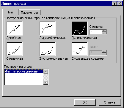
Rice. 3. Option “Trend lines”
The use of other types of trend (logarithmic, power, exponential, moving average) also does not give such an effective result. They unsatisfactorily approximate the actual values, their coefficients of determination are negligible:
- logarithmic R2 = 0.0166;
- power R 2 =0.0197;
- exponential R 2 =8E-05.
2. Subtracting trend values from actual sales volumes , we determine the magnitude of the seasonal component, using the MS Excel application package (Fig. 4).
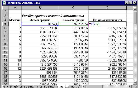
Rice. 4. Calculation of seasonal component values in MS Excel.
Table 2.
Calculation of seasonal component values
|
Months |
Volume of sales |
Trend value |
Seasonal component |
Let us adjust the values of the seasonal component so that their sum is equal to zero.
Table 3.
Calculation of average values of the seasonal component
|
Months |
Seasonal component |
||||
3. We calculate model errors as the difference between actual values and model values.
Table 4.
Error calculation
|
Month |
Volume of sales |
Model value |
Deviations |
We find the root mean square error of the model (E) using the formula:
E= Σ O 2: Σ (T+S) 2
Where:
T- trend value of sales volume;
S
– seasonal component;
ABOUT
- deviations of the model from actual values
E= 0.003739 or 0.37%
The magnitude of the error obtained allows us to say that the constructed model well approximates the actual data, i.e. it fully reflects the economic trends that determine sales volume and is a prerequisite for building high-quality forecasts.
Let's build a forecasting model:
The constructed model is presented graphically in Fig. 5.
5. Based on the model, we build a final forecast of sales volume. To mitigate the influence of past trends on the reliability of the forecast model, it is proposed to combine trend analysis with exponential smoothing. This will eliminate the lack of adaptive models, i.e. take into account emerging new economic trends:
F pr t = a F f t-1 + (1-a) F m t
Where:
F pr t - forecast value of sales volume;
F f t-1
– actual value of sales volume in the previous year;
F m t
- value of the model;
A
– smoothing constant.
It is recommended to determine the smoothing constant using the method of expert assessments as the probability of maintaining the existing market conditions, i.e. if the main characteristics change / fluctuate at the same speed / amplitude as before, then there are no prerequisites for a change in market conditions, and therefore a ® 1, if vice versa, then a ® 0.
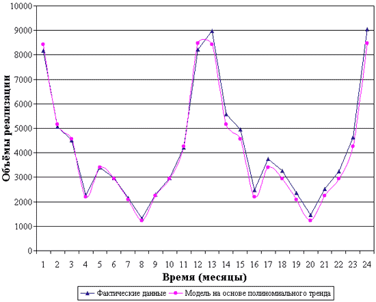
Rice. 5. Sales volume forecast model
Thus, the forecast for January of the third season is determined as follows.
We determine the predicted value of the model:
F m t = 1,924.92 + 162.44 =2087 ± 7.8 (rub.)
Actual sales volume in the previous year (F f t-1) amounted to 2,361 rubles. We accept a smoothing coefficient of 0.8. Let's get the forecast sales volume:
F pr t = 0.8*2,361 + (1-0.8) *2087 = 2306.2 (rub.)
In addition, to increase the reliability of the forecast, it is recommended to build all possible forecast scenarios and calculate the confidence interval of the forecast.
Dmitriev Mikhail Nikolaevich, Head of the Department of Economics and Entrepreneurship of the Nizhny Novgorod University of Architecture and Civil Engineering (NNGASU), Doctor of Economic Sciences, Professor.
Address: 603000, N. Novgorod, st. Gorkogo, 142a, apt. 25.
Tel. 37-92-19 (home) 30-54-37 (work)
Koshechkin Sergey Aleksandrovich, Candidate of Economic Sciences, senior lecturer Lecturer at the Department of Economics and Entrepreneurship at the Nizhny Novgorod University of Architecture and Civil Engineering (NNGASU).
Address: 603148, N. Novgorod, st. Chaadaeva, 48, apt. 39.
Tel. 46-79-20 (home) 30-53-49 (work)