A system of linear equations is a union of n linear equations, each containing k variables. It is written like this:
Many, when encountering higher algebra for the first time, mistakenly believe that the number of equations must necessarily coincide with the number of variables. In school algebra this usually happens, but for higher algebra this is generally not true.
The solution to a system of equations is a sequence of numbers (k 1, k 2, ..., k n), which is the solution to each equation of the system, i.e. when substituting into this equation instead of the variables x 1, x 2, ..., x n gives the correct numerical equality.
Accordingly, solving a system of equations means finding the set of all its solutions or proving that this set is empty. Since the number of equations and the number of unknowns may not coincide, three cases are possible:
- The system is inconsistent, i.e. the set of all solutions is empty. A rather rare case that is easily detected no matter what method is used to solve the system.
- The system is consistent and determined, i.e. has exactly one solution. Classic version, well known since school days.
- The system is consistent and undefined, i.e. has infinitely many solutions. This is the toughest option. It is not enough to indicate that “the system has an infinite set of solutions” - it is necessary to describe how this set is structured.
A variable x i is called allowed if it is included in only one equation of the system, and with a coefficient of 1. In other words, in other equations the coefficient of the variable x i must be equal to zero.
If we select one allowed variable in each equation, we obtain a set of allowed variables for the entire system of equations. The system itself, written in this form, will also be called resolved. Generally speaking, one and the same original system can be reduced to different permitted ones, but for now we are not concerned about this. Here are examples of permitted systems:
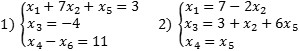
Both systems are resolved with respect to the variables x 1 , x 3 and x 4 . However, with the same success it can be argued that the second system is resolved with respect to x 1, x 3 and x 5. It is enough to rewrite the very last equation in the form x 5 = x 4.
Now let's consider a more general case. Let us have k variables in total, of which r are allowed. Then two cases are possible:
- The number of allowed variables r is equal to the total number of variables k: r = k. We obtain a system of k equations in which r = k allowed variables. Such a system is joint and definite, because x 1 = b 1, x 2 = b 2, ..., x k = b k;
- The number of allowed variables r is less total number variables k : r< k . Остальные (k − r ) переменных называются свободными - они могут принимать любые значения, из которых легко вычисляются разрешенные переменные.
So, in the above systems, the variables x 2, x 5, x 6 (for the first system) and x 2, x 5 (for the second) are free. The case when there are free variables is better formulated as a theorem:
Please note: this is very important point! Depending on how you write the resulting system, the same variable can be either allowed or free. Most tutors higher mathematics It is recommended to write out variables in lexicographical order, i.e. ascending index. However, you are under no obligation to follow this advice.
Theorem. If in a system of n equations the variables x 1, x 2, ..., x r are allowed, and x r + 1, x r + 2, ..., x k are free, then:
- If we set the values of the free variables (x r + 1 = t r + 1, x r + 2 = t r + 2, ..., x k = t k), and then find the values x 1, x 2, ..., x r, we get one of decisions.
- If in two solutions the values of free variables coincide, then the values of allowed variables also coincide, i.e. solutions are equal.
What is the meaning of this theorem? To obtain all solutions to a resolved system of equations, it is enough to isolate the free variables. Then, assigning to free variables different meanings, we will receive ready-made solutions. That's all - in this way you can get all the solutions of the system. There are no other solutions.
Conclusion: the resolved system of equations is always consistent. If the number of equations in a resolved system is equal to the number of variables, the system will be definite; if less, it will be indefinite.
And everything would be fine, but the question arises: how to obtain a resolved one from the original system of equations? For this there is
Systems of equations have been widely used in the economic industry with mathematical modeling various processes. For example, when solving problems of production management and planning, logistics routes (transport problem) or equipment placement.
Systems of equations are used not only in mathematics, but also in physics, chemistry and biology, when solving problems of finding population size.
A system of linear equations is two or more equations with several variables for which it is necessary to find a common solution. Such a sequence of numbers for which all equations become true equalities or prove that the sequence does not exist.
Linear equation
Equations of the form ax+by=c are called linear. The designations x, y are the unknowns whose value must be found, b, a are the coefficients of the variables, c is the free term of the equation.
Solving an equation by plotting it will look like a straight line, all points of which are solutions to the polynomial.
Types of systems of linear equations
The simplest examples are considered to be systems of linear equations with two variables X and Y.
F1(x, y) = 0 and F2(x, y) = 0, where F1,2 are functions and (x, y) are function variables.
Solve system of equations - this means finding values (x, y) at which the system turns into a true equality or establishing that suitable values x and y do not exist.
A pair of values (x, y), written as the coordinates of a point, is called a solution to a system of linear equations.
If systems have one common solution or no solution exists, they are called equivalent.
Homogeneous systems of linear equations are systems whose right-hand side is equal to zero. If the right part after the equal sign has a value or is expressed by a function, such a system is heterogeneous.
The number of variables can be much more than two, then we should talk about an example of a system of linear equations with three or more variables.
When faced with systems, schoolchildren assume that the number of equations must necessarily coincide with the number of unknowns, but this is not the case. The number of equations in the system does not depend on the variables; there can be as many of them as desired.
Simple and complex methods for solving systems of equations
There is no general analytical method for solving such systems; all methods are based on numerical solutions. The school mathematics course describes in detail such methods as permutation, algebraic addition, substitution, as well as graphical and matrix methods, solution by the Gaussian method.
The main task when teaching solution methods is to teach how to correctly analyze the system and find the optimal solution algorithm for each example. The main thing is not to memorize a system of rules and actions for each method, but to understand the principles of using a particular method
Solving examples of systems of linear equations of the 7th grade program secondary school quite simple and explained in great detail. In any mathematics textbook, this section is given enough attention. Solving examples of systems of linear equations using the Gauss and Cramer method is studied in more detail in the first years of higher education.
Solving systems using the substitution method
The actions of the substitution method are aimed at expressing the value of one variable in terms of the second. The expression is substituted into the remaining equation, then it is reduced to a form with one variable. The action is repeated depending on the number of unknowns in the system
Let us give a solution to an example of a system of linear equations of class 7 using the substitution method:

As can be seen from the example, the variable x was expressed through F(X) = 7 + Y. The resulting expression, substituted into the 2nd equation of the system in place of X, helped to obtain one variable Y in the 2nd equation. Solution this example does not cause difficulties and allows you to obtain the Y value. Last step This is a check of the received values.
It is not always possible to solve an example of a system of linear equations by substitution. The equations can be complex and expressing the variable in terms of the second unknown will be too cumbersome for further calculations. When there are more than 3 unknowns in the system, solving by substitution is also inappropriate.
Solution of an example of a system of linear inhomogeneous equations:

Solution using algebraic addition
When searching for solutions to systems using the addition method, they perform term-by-term addition and multiplication of equations by different numbers. The ultimate goal of mathematical operations is an equation in one variable.

Application of this method requires practice and observation. Solving a system of linear equations using the addition method when there are 3 or more variables is not easy. Algebraic addition is convenient to use when equations contain fractions and decimals.
Solution algorithm:
- Multiply both sides of the equation by a certain number. As a result arithmetic action one of the coefficients of the variable must become equal to 1.
- Add the resulting expression term by term and find one of the unknowns.
- Substitute the resulting value into the 2nd equation of the system to find the remaining variable.
Method of solution by introducing a new variable
A new variable can be introduced if the system requires finding a solution for no more than two equations; the number of unknowns should also be no more than two.
The method is used to simplify one of the equations by introducing a new variable. The new equation is solved for the introduced unknown, and the resulting value is used to determine the original variable.

The example shows that by introducing a new variable t, it was possible to reduce the 1st equation of the system to the standard one quadratic trinomial. You can solve a polynomial by finding the discriminant.
It is necessary to find the value of the discriminant using the well-known formula: D = b2 - 4*a*c, where D is the desired discriminant, b, a, c are the factors of the polynomial. In the given example, a=1, b=16, c=39, therefore D=100. If the discriminant Above zero, then there are two solutions: t = -b±√D / 2*a, if the discriminant less than zero, then there is only one solution: x= -b / 2*a.
The solution for the resulting systems is found by the addition method.
Visual method for solving systems
Suitable for 3 equation systems. The method consists in constructing graphs of each equation included in the system on the coordinate axis. The coordinates of the points of intersection of the curves and will be general decision systems.
The graphical method has a number of nuances. Let's look at several examples of solving systems of linear equations in a visual way.

As can be seen from the example, for each line two points were constructed, the values of the variable x were chosen arbitrarily: 0 and 3. Based on the values of x, the values for y were found: 3 and 0. Points with coordinates (0, 3) and (3, 0) were marked on the graph and connected by a line.
The steps must be repeated for the second equation. The point of intersection of the lines is the solution of the system.
The following example requires finding a graphical solution to a system of linear equations: 0.5x-y+2=0 and 0.5x-y-1=0.

As can be seen from the example, the system has no solution, because the graphs are parallel and do not intersect along their entire length.

The systems from examples 2 and 3 are similar, but when constructed it becomes obvious that their solutions are different. It should be remembered that it is not always possible to say whether a system has a solution or not; it is always necessary to construct a graph.
The matrix and its varieties
Matrices are used for short note systems of linear equations. A matrix is a table special type filled with numbers. n*m has n - rows and m - columns.
A matrix is square when the number of columns and rows are equal. A matrix-vector is a matrix of one column with an infinitely possible number of rows. A matrix with ones along one of the diagonals and other zero elements is called identity.
An inverse matrix is a matrix when multiplied by which the original one turns into a unit matrix; such a matrix exists only for the original square one.
Rules for converting a system of equations into a matrix
In relation to systems of equations, the coefficients and free terms of the equations are written as matrix numbers; one equation is one row of the matrix.
A matrix row is said to be nonzero if at least one element of the row is not zero. Therefore, if in any of the equations the number of variables differs, then it is necessary to enter zero in place of the missing unknown.
The matrix columns must strictly correspond to the variables. This means that the coefficients of the variable x can be written only in one column, for example the first, the coefficient of the unknown y - only in the second.
When multiplying a matrix, all elements of the matrix are sequentially multiplied by a number.
Options for finding the inverse matrix
The formula for finding the inverse matrix is quite simple: K -1 = 1 / |K|, where K -1 - inverse matrix, and |K| is the determinant of the matrix. |K| must not be equal to zero, then the system has a solution.
The determinant is easily calculated for a two-by-two matrix; you just need to multiply the diagonal elements by each other. For the “three by three” option, there is a formula |K|=a 1 b 2 c 3 + a 1 b 3 c 2 + a 3 b 1 c 2 + a 2 b 3 c 1 + a 2 b 1 c 3 + a 3 b 2 c 1 . You can use the formula, or you can remember that you need to take one element from each row and each column so that the numbers of columns and rows of elements are not repeated in the work.
Solving examples of systems of linear equations using the matrix method
The matrix method of finding a solution allows you to reduce cumbersome entries when solving systems with a large number of variables and equations.

In the example, a nm are the coefficients of the equations, the matrix is a vector x n are variables, and b n are free terms.


Solving systems using the Gaussian method
In higher mathematics, the Gaussian method is studied together with the Cramer method, and the process of finding solutions to systems is called the Gauss-Cramer solution method. These methods are used to find variables of systems with a large number of linear equations.
The Gauss method is very similar to solutions by substitution and algebraic addition, but is more systematic. In the school course, the solution by the Gaussian method is used for systems of 3 and 4 equations. The purpose of the method is to reduce the system to the form of an inverted trapezoid. By means of algebraic transformations and substitutions, the value of one variable is found in one of the equations of the system. The second equation is an expression with 2 unknowns, while 3 and 4 are, respectively, with 3 and 4 variables.
After bringing the system to the described form, the further solution is reduced to the sequential substitution of known variables into the equations of the system.
In school textbooks for grade 7, an example of a solution by the Gauss method is described as follows:

As can be seen from the example, at step (3) two equations were obtained: 3x 3 -2x 4 =11 and 3x 3 +2x 4 =7. Solving any of the equations will allow you to find out one of the variables x n.

Theorem 5, which is mentioned in the text, states that if one of the equations of the system is replaced by an equivalent one, then the resulting system will also be equivalent to the original one.
The Gaussian method is difficult for students to understand high school, but is one of the most interesting ways to develop the ingenuity of children studying under the program in-depth study in math and physics classes.
For ease of recording, calculations are usually done as follows:

The coefficients of the equations and free terms are written in the form of a matrix, where each row of the matrix corresponds to one of the equations of the system. separates the left side of the equation from the right. Roman numerals indicate the numbers of equations in the system.
First, write down the matrix to be worked with, then all the actions carried out with one of the rows. The resulting matrix is written after the "arrow" sign and the necessary algebraic operations are continued until the result is achieved.
The result should be a matrix in which one of the diagonals is equal to 1, and all other coefficients are equal to zero, that is, the matrix is reduced to a unit form. We must not forget to perform calculations with numbers on both sides of the equation.
This recording method is less cumbersome and allows you not to be distracted by listing numerous unknowns.
The free use of any solution method will require care and some experience. Not all methods are of an applied nature. Some methods of finding solutions are more preferable in a particular area of human activity, while others exist for educational purposes.
When solving linear equations, we strive to find the root, that is, the value for the variable that will turn the equation into a correct equality.
To find the root of the equation you need equivalent transformations bring the equation given to us to the form
\(x=[number]\)
This number will be the root.
That is, we transform the equation, making it simpler with each step, until we reduce it to a completely primitive equation “x = number”, where the root is obvious. The most frequently used transformations when solving linear equations are the following:
For example: add \(5\) to both sides of the equation \(6x-5=1\)
\(6x-5=1\) \(|+5\)
\(6x-5+5=1+5\)
\(6x=6\)
Please note that we could get the same result faster by simply writing the five on the other side of the equation and changing its sign. Actually, this is exactly how the school “transfer through equals with a change of sign to the opposite” is done.
2. Multiplying or dividing both sides of an equation by the same number or expression.
For example: divide the equation \(-2x=8\) by minus two
\(-2x=8\) \(|:(-2)\)
\(x=-4\)
Typically this step is performed at the very end, when the equation has already been reduced to the form \(ax=b\), and we divide by \(a\) to remove it from the left.
3. Using the properties and laws of mathematics: opening parentheses, bringing similar terms, reducing fractions, etc.
Add \(2x\) left and right
Subtract \(24\) from both sides of the equation
We present similar terms again
Now we divide the equation by \(-3\), thereby removing the front X on the left side.
Answer : \(7\)
The answer has been found. However, let's check it out. If seven is really a root, then substituting it instead of X into the original equation should result in the correct equality - same numbers left and right. Let's try.
Examination:
\(6(4-7)+7=3-2\cdot7\)
\(6\cdot(-3)+7=3-14\)
\(-18+7=-11\)
\(-11=-11\)
It worked out. This means that seven is indeed the root of the original linear equation.
Don’t be lazy to check the answers you found by substitution, especially if you are solving an equation on a test or exam.
The question remains - how to determine what to do with the equation at the next step? How exactly to convert it? Divide by something? Or subtract? And what exactly should I subtract? Divide by what?
The answer is simple:
Your goal is to bring the equation to the form \(x=[number]\), that is, on the left is x without coefficients and numbers, and on the right is only a number without variables. Therefore, look at what is stopping you and do the opposite of what the interfering component does.
To better understand this, let's look at the solution of the linear equation \(x+3=13-4x\) step by step.
Let's think: how does this equation differ from \(x=[number]\)? What's stopping us? What's wrong?
Well, firstly, the three interferes, since on the left there should be only a lone X, without numbers. What does the troika “do”? Added to X. So, to remove it - subtract the same three. But if we subtract three from the left, we must subtract it from the right so that the equality is not violated.
\(x+3=13-4x\) \(|-3\)
\(x+3-3=13-4x-3\)
\(x=10-4x\)
Fine. Now what's stopping you? \(4x\) on the right, because there should only be numbers there. \(4x\) deducted- we remove by adding.
\(x=10-4x\) \(|+4x\)
\(x+4x=10-4x+4x\)
Now we present similar terms on the left and right.
It's almost ready. All that remains is to remove the five on the left. What is she doing"? Multiplies on x. So let's remove it division.
\(5x=10\) \(|:5\)
\(\frac(5x)(5)\) \(=\)\(\frac(10)(5)\)
\(x=2\)
The solution is complete, the root of the equation is two. You can check by substitution.
notice, that most often there is only one root in linear equations. However, two special cases may occur.
Special case 1 – there are no roots in a linear equation.
Example . Solve the equation \(3x-1=2(x+3)+x\)
Solution :
Answer : no roots.
In fact, the fact that we will come to such a result was visible earlier, even when we received \(3x-1=3x+6\). Think about it: how can \(3x\) from which we subtracted \(1\), and \(3x\) to which we added \(6\) be equal? Obviously, no way, because they did the same thing different actions! It is clear that the results will vary.
Special case 2 – a linear equation has an infinite number of roots.
Example . Solve linear equation \(8(x+2)-4=12x-4(x-3)\)Solution :
Answer : any number.
This, by the way, was noticeable even earlier, at the stage: \(8x+12=8x+12\). Indeed, left and right are the same expressions. Whatever X you substitute, it will be the same number both there and there.
More complex linear equations.
The original equation does not always immediately look like linear; sometimes it is “masked” as other, more complex equations. However, in the process of transformation, the disguise disappears.
Example . Find the root of the equation \(2x^(2)-(x-4)^(2)=(3+x)^(2)-15\)
Solution :
|
\(2x^(2)-(x-4)^(2)=(3+x)^(2)-15\) |
It would seem that there is an x squared here - this is not a linear equation! But don't rush. Let's apply |
|
|
\(2x^(2)-(x^(2)-8x+16)=9+6x+x^(2)-15\) |
Why is the expansion result \((x-4)^(2)\) in parentheses, but the result \((3+x)^(2)\) is not? Because there is a minus in front of the first square, which will change all the signs. And in order not to forget about this, we take the result in brackets, which we now open. |
|
|
\(2x^(2)-x^(2)+8x-16=9+6x+x^(2)-15\) |
We present similar terms |
|
|
\(x^(2)+8x-16=x^(2)+6x-6\) |
||
|
\(x^(2)-x^(2)+8x-6x=-6+16\) |
We present similar ones again. |
|
|
Like this. It turns out that the original equation is quite linear, and the X squared is nothing more than a screen to confuse us. :) We complete the solution by dividing the equation by \(2\), and we get the answer. |
Answer : \(x=5\)
Example . Solve linear equation \(\frac(x+2)(2)\) \(-\) \(\frac(1)(3)\) \(=\) \(\frac(9+7x)(6 )\)
Solution :
|
\(\frac(x+2)(2)\) \(-\) \(\frac(1)(3)\) \(=\) \(\frac(9+7x)(6)\) |
The equation doesn’t look linear, it’s some kind of fractions... However, let’s get rid of the denominators by multiplying both sides of the equation by the common denominator of all – six |
|
|
\(6\cdot\)\((\frac(x+2)(2)\) \(-\) \(\frac(1)(3))\) \(=\) \(\frac( 9+7x)(6)\) \(\cdot 6\) |
Expand the bracket on the left |
|
|
\(6\cdot\)\(\frac(x+2)(2)\) \(-\) \(6\cdot\)\(\frac(1)(3)\) \(=\) \(\frac(9+7x)(6)\) \(\cdot 6\) |
Now let's reduce the denominators |
|
|
\(3(x+2)-2=9+7x\) |
Now it looks like a regular linear one! Let's finish it. |
|
|
By translating through equals we collect X's on the right and numbers on the left |
||
|
Well, dividing the right and left sides by \(-4\), we get the answer |
Answer : \(x=-1.25\)
In this article we will consider the principle of solving such equations as linear equations. Let us write down the definition of these equations and set general form. We will analyze all the conditions for finding solutions to linear equations, using, among other things, practical examples.
Please note that the material below contains information on linear equations with one variable. Linear equations in two variables are discussed in a separate article.
Yandex.RTB R-A-339285-1
What is a linear equation
Definition 1Linear equation is an equation written as follows:
a x = b, Where x– variable, a And b- some numbers.
This formulation was used in the algebra textbook (7th grade) by Yu.N. Makarychev.
Example 1
Examples of linear equations would be:
3 x = 11(equation with one variable x at a = 5 And b = 10);
− 3 , 1 y = 0 ( linear equation with variable y, Where a = - 3, 1 And b = 0);
x = − 4 And − x = 5.37(linear equations, where the number a written explicitly and equal to 1 and - 1, respectively. For the first equation b = - 4 ; for the second - b = 5.37) and so on.
In different educational materials There may be different definitions. For example, Vilenkin N.Ya. Linear equations also include those equations that can be transformed into the form a x = b by transferring terms from one part to another with a change of sign and bringing similar terms. If we follow this interpretation, the equation 5 x = 2 x + 6 – also linear.
But the algebra textbook (7th grade) by Mordkovich A.G. gives the following description:
Definition 2
A linear equation in one variable x is an equation of the form a x + b = 0, Where a And b– some numbers called coefficients of a linear equation.
Example 2
An example of linear equations of this type could be:
3 x − 7 = 0 (a = 3 , b = − 7) ;
1, 8 y + 7, 9 = 0 (a = 1, 8, b = 7, 9).
But there are also examples of linear equations that we have already used above: of the form a x = b, For example, 6 x = 35.
We will immediately agree that in this article by a linear equation with one variable we will understand the equation written a x + b = 0, Where x– variable; a, b – coefficients. We see this form of a linear equation as the most justified, since linear equations are algebraic equations of the first degree. And the other equations indicated above, and the equations given by equivalent transformations in the form a x + b = 0, we define as equations that reduce to linear equations.
With this approach, the equation 5 x + 8 = 0 is linear, and 5 x = − 8- an equation that reduces to a linear one.
Principle of solving linear equations
Let's look at how to determine whether a given linear equation will have roots and, if so, how many and how to determine them.
Definition 3
The fact of the presence of roots of a linear equation is determined by the values of the coefficients a And b. Let's write down these conditions:
- at a ≠ 0 linear equation has a single root x = - b a ;
- at a = 0 And b ≠ 0 a linear equation has no roots;
- at a = 0 And b = 0 a linear equation has infinitely many roots. Essentially in in this case any number can become the root of a linear equation.
Let's give an explanation. We know that in the process of solving an equation it is possible to transform a given equation into an equivalent one, which means that it has the same roots as the original equation, or also has no roots. We can make the following equivalent transformations:
- transfer a term from one part to another, changing the sign to the opposite;
- multiply or divide both sides of an equation by the same number that is not zero.
Thus, we transform the linear equation a x + b = 0, moving the term b from left to right side with a change of sign. We get: a · x = − b .
So, we divide both sides of the equation by a non-zero number A, resulting in an equality of the form x = - b a . That is, when a ≠ 0, original equation a x + b = 0 is equivalent to the equality x = - b a, in which the root - b a is obvious.
By contradiction it is possible to demonstrate that the root found is the only one. Let us designate the found root - b a as x 1 . Let us assume that there is another root of the linear equation with the designation x 2 . And of course: x 2 ≠ x 1, and this, in turn, based on the definition of equal numbers through the difference, is equivalent to the condition x 1 − x 2 ≠ 0 . Taking into account the above, we can create the following equalities by substituting the roots:
a x 1 + b = 0 and a x 2 + b = 0.
The property of numerical equalities makes it possible to perform term-by-term subtraction of parts of equalities:
a x 1 + b − (a x 2 + b) = 0 − 0, from here: a · (x 1 − x 2) + (b − b) = 0 and onwards a · (x 1 − x 2) = 0 . Equality a · (x 1 − x 2) = 0 is incorrect because it was previously specified that a ≠ 0 And x 1 − x 2 ≠ 0 . The resulting contradiction serves as proof that when a ≠ 0 linear equation a x + b = 0 has only one root.
Let us justify two more clauses of the conditions containing a = 0 .
When a = 0 linear equation a x + b = 0 will be written as 0 x + b = 0. The property of multiplying a number by zero gives us the right to assert that whatever number is taken as x, substituting it into equality 0 x + b = 0, we get b = 0 . The equality is valid for b = 0; in other cases, when b ≠ 0, equality becomes false.
So when a = 0 and b = 0 , any number can become the root of a linear equation a x + b = 0, since when these conditions are met, substituting instead x any number, we get the correct numerical equality 0 = 0 . When a = 0 And b ≠ 0 linear equation a x + b = 0 will not have roots at all, since when executing specified conditions, substituting instead x any number, we get an incorrect numerical equality b = 0.
All the above considerations give us the opportunity to write down an algorithm that makes it possible to find a solution to any linear equation:
- by the type of record we determine the values of the coefficients a And b and analyze them;
- at a = 0 And b = 0 the equation will have infinitely many roots, i.e. any number will become the root of the given equation;
- at a = 0 And b ≠ 0
- at a, different from zero, we begin searching for the only root of the original linear equation:
- let's move the coefficient b to the right side with a change of sign to the opposite, bringing the linear equation to the form a · x = − b ;
- divide both sides of the resulting equality by the number a, which will give us the desired root of the given equation: x = - b a.
Actually, the described sequence of actions is the answer to the question of how to find a solution to a linear equation.
Finally, let us clarify that equations of the form a x = b are solved using a similar algorithm with the only difference that the number b in such a notation has already been transferred to the required part of the equation, and with a ≠ 0 you can immediately divide the parts of an equation by a number a.
Thus, to find a solution to the equation a x = b, we use the following algorithm:
- at a = 0 And b = 0 the equation will have infinitely many roots, i.e. any number can become its root;
- at a = 0 And b ≠ 0 the given equation will have no roots;
- at a, not equal to zero, both sides of the equation are divided by the number a, which makes it possible to find the only root that is equal to b a.
Examples of solving linear equations
Example 3Linear equation needs to be solved 0 x − 0 = 0.
Solution
By writing the given equation we see that a = 0 And b = − 0(or b = 0, which is the same). Thus, a given equation can have an infinite number of roots or any number.
Answer: x– any number.
Example 4
It is necessary to determine whether the equation has roots 0 x + 2, 7 = 0.
Solution
From the record we determine that a = 0, b = 2, 7. Thus, the given equation will have no roots.
Answer: the original linear equation has no roots.
Example 5
Given a linear equation 0.3 x − 0.027 = 0. It needs to be resolved.
Solution
By writing the equation we determine that a = 0, 3; b = - 0.027, which allows us to assert that the given equation has a single root.
Following the algorithm, we move b to the right side of the equation, changing the sign, we get: 0.3 x = 0.027. Next, we divide both sides of the resulting equality by a = 0, 3, then: x = 0, 027 0, 3.
Let's divide decimal fractions:
0.027 0.3 = 27 300 = 3 9 3 100 = 9 100 = 0.09
The result obtained is the root of the given equation.
Let us briefly write the solution as follows:
0.3 x - 0.027 = 0.0.3 x = 0.027, x = 0.027 0.3, x = 0.09.
Answer: x = 0.09.
For clarity, we present the solution to the writing equation a x = b.
Example N
The given equations are: 1) 0 x = 0 ; 2) 0 x = − 9 ; 3) - 3 8 x = - 3 3 4 . They need to be resolved.
Solution
All given equations records correspond a x = b. Let's look at them one by one.
In the equation 0 x = 0, a = 0 and b = 0, which means: any number can be the root of this equation.
In the second equation 0 x = − 9: a = 0 and b = − 9, thus, this equation will have no roots.
Based on the form of the last equation - 3 8 · x = - 3 3 4, we write the coefficients: a = - 3 8, b = - 3 3 4, i.e. the equation has a single root. Let's find him. Let's divide both sides of the equation by a, resulting in: x = - 3 3 4 - 3 8. Simplify the fraction using the division rule negative numbers followed by translation mixed number V common fraction and dividing ordinary fractions:
3 3 4 - 3 8 = 3 3 4 3 8 = 15 4 3 8 = 15 4 8 3 = 15 8 4 3 = 10
Let us briefly write the solution as follows:
3 8 · x = - 3 3 4 , x = - 3 3 4 - 3 8 , x = 10 .
Answer: 1) x– any number, 2) the equation has no roots, 3) x = 10.
If you notice an error in the text, please highlight it and press Ctrl+Enter